Comparative Analysis of Dispersion Parameter Estimates in Loglinear Modeling

Transcription

1 Comparative Analysis of Dispersion Parameter Estimates in Loglinear Modeling Applied to E-commerce Sales and Customer Data SENIOR PROJECT PRESENTED TO THE FACULTY OF THE STATISTICS DEPARTMENT CALIFORNIA POLYTECHNIC STATE UNIVERSITY, SAN LUIS OBISPO IN PARTIAL FULFILLMENT OF THE REQUIREMENTS FOR THE DEGREE OF BACHELOR OF SCIENCE SCOTT DAVIS DR. SAMUEL FRAME, ADVISOR SEPTEMBER 2012 Abstract When loglinear models are applied to count data the issue of over-dispersion often arises. Moment and maximum likelihood estimation methods in accounting for over-dispersion are widely used because they allow for model checking tools such as Chi-square, F, and likelihood ratio tests. Herein is a comparison between R functions that each uses one method; glm.nb uses MLE, and glm.poisson.disp uses MME. The Index of Dissimilarity and visual model selection (ECDF plots) are also incorporated. These are applied to sales data using product and customer information compiled over the last five years that was generously provided by an e-commerce company.

2 1 P age

3 Contents 1. Introduction Background Data & Methods The Data Methods Functions Over-dispersion Model Fit Dissimilarity Visual Model Fit Model Assumptions Differing Model Results Results Discussion Conclusion References Appendix 1-A Model Comparisons: Odds Ratios (95% CI) Appendix 1-B: glm.nb B.1: Residual Diagnostics B.2: Univariate standardized deviance residual boxplots (Sex, Income, and Brand) B.3: Univariate standardized deviance residual boxplots (Channel, Cordless, and Condition) B.4: DF Beta Plots Appendix 1-C: glm.poisson.disp C.1: Residual Diagnostics C.2: Univariate standardized deviance residual boxplots (Sex, Income, and Brand) C.3: Univariate standardized deviance residual boxplots (Channel, Cordless, and Condition) C.4: DF Beta Plots Appendix A: ANOVA Output B.1: Summary() Output glm.nb B.2: Summary() Output glm.poisson.disp P age

4 Figure 1. Distribution of counts of covariate frequencies Figure 2. ECDF of all models Figure 3. Observed and expected frequencies vs. Sales Volume Figure 4. Deviance residuals for both models are approximately normally distributed Table 1. Listing of variable names and levels Table 2. 2-Way interactions included in both models Table 3. Test of over-dispersion results Table 4. Dissimilarity index values. Smaller values indicate better fit Table 5. Deviance and fit statistics for all fitted models Table 6. Inestimable parameters for both models Table 7. Interactions showing negative associations Table 8. Model comparisons Table 9. Additional parameters output by glm.nb P age

5 1. Introduction For data that is well represented in a contingency table, by a table of counts, or where there is not a distinct response variable, loglinear modeling is commonly employed to describe the direction and magnitude of association between variables (Agresti 2007, Venables & Ripley 2002, McCullagh & Nelder 1989). It is especially useful for higher-order models or when the variables have many levels. All of the above describe the data analyzed herein. See Jansakul and Hinde for a listing field application and authors. These data are sales data provided by an e-commerce company and include a wide variety of products with mass appeal. As such, the sales frequencies for the many combinations of covariates can be vastly different from one another. Such large differences make it difficult to account for the variance between different covariate combinations. From the Comprehensive R Archive Network (CRAN, comes two functions used to model such data: glm.poisson.disp() (in dispmod; Luca Scrucca 2012, Breslow, N.E. 1984) and glm.nb() (in MASS; Venables, W. N. and Ripley, B. D. 2002). While both model the data in valid ways glm.poisson.disp() using a Method of Moment (MM) estimator of the parameters, and glm.nb() using Maximum Likelihood (ML) and fit this data very well, they often give opposing directions of association for covariate combinations. This paper briefly discusses the effect on the model from using both R functions and the implications on inference if one is chosen in lieu of another. In addition, results for the main research questions pertinent to the company whose data are used are addressed in depth. The layout of the paper begins with a description of how the project came about, the data and methods used with a description of the R functions used and a brief of over-dispersion, followed up with a section on model fitting, a discussion of some issues encountered, the results of the sales data, and the summary. 4 P age

6 2. Background In proposing the use of these data for this project, two areas of interest arose. The main question of interest centered on what may influence how long an item stays in inventory of the company. Another aim was to measure how, and in what way, the variables related to one another. However, these data restricted direct analysis of this question because of the way avg days in inv is calculated. It is an average of the days in inventory for all of the items of a specific type received by the warehouse for any of the drops to the warehouse (a drop occurs twice a day and is when the system that processes orders releases them to the warehouse for fulfillment). As such, this value may incorporate storage time from different/multiple supplier shipments to the warehouse. Also, without distinction for items that are drop shipped or pre-sale (put on sale before being received to the warehouse), there is no clear way to distinguish in this analysis and beyond summary statistics if, or in what way, the average days in inventory is affected by the characteristics of products or customers. Also, with respect to storage time, because the data do not make distinctions among unique customers, there is no way to analyze differences between specific combinations of customer characteristics related to particular products. Thus, any interpretations of results from such an investigation may be spurious. However, what was able to be addressed was the strength and direction of associations between a selected subset of variables. 5 P age

7 3. Data & Methods 3.1 The Data The original data file contained 1,186,929 observations. Each observation contains up to 25 variable descriptions. From this file, SAS 9.2 was used for data management, reducing the number of variables to six whose unique non-zero combinations were counted and exported using PROC SQL with analysis carried out using R There are 2,490 such combinations whose frequencies are studied. Below are the descriptions of the variable of interest. Each product manufacturer is listed under Brand. Channel refers to the sales channel that the product is sold through. Agg_channel is comprised of Club CPO: Phone, Club CPO: Web, Other, Outlets: Phone, Outlets: Web, Press.Wash: Phone, Press.Wash: Web, Reconditioned Tools: Web, Reconditioned Tools: Phone, Tool Crib: Phone, Tool Crib: Web, and Wholesale. A customer s gender is given by Sex, and the original levels were aggregated as follows: unknown and ambiguous as Unknown; female and probably female as Female; male and probably male as Male. A product s sales condition is either New or Reconditioned. The descriptions for a tool being cordless or corded are obvious. Brand Black & Decker Fein Makita Powermatic Bosch (Ref level) Festool Ridgid Bostitch Homelite Milwaukee Ryobi Campbell Hausfeld Jet Metabo Channel Panasonic Senco Delta Karcher Porter Cable Skil Dewalt agg_channel Branded Web (Ref level) Sex Unknown Female Income Cordless High ($75k- 200k+) Cordless (Ref level) Middle ($30k-75k) (Ref level) Not Cordless Condition New (Ref level) Reconditioned Phone Amazon Sales ebay Sales Male (Ref level) Low (-$10k-20k) Table 1. Listing of variable names and levels. 3.2 Methods For data that is well represented in contingency tables, loglinear modeling may be employed as a way to assess associations between any, or all, of the variables under consideration. Loglinear models extend inference beyond 2-way contingency tables to multi-way tables where the conditional relationship between two or more discrete, categorical variables is analyzed by taking the natural logarithm of the cell 6 P age

8 frequencies. It allows for interpretations of the strength and direction of relationships in these tables. What is being modeled is the estimated effect on the frequency by unique groupings as shown by the strength of the association between one or more variables in each group. As is the case in this analysis where we have multiple two-variable interactions, the association between any two variables, given some fixed level of the other four variables, has either a positive or negative effect on the expected number of times this unique grouping appears in the data set. It may also be said that the effect on the estimated cell frequency of one customer-product specification is x-times higher or lower when compared to the reference group. Often, due to the complexity of interpretations or relevance, only one variable level at a time will be adjusted. For instance, to compare different brands the remaining five variable levels will remain the same for both brands; given these fixed levels, Brand A is associated with an increase (decrease) in the estimated odds of a sale compared to Brand B. The Poisson distribution assumes the mean and variance of the response are equal. The extra-variation, referred to as extra-dispersion (in this case, strictly over-dispersion), inherent in this data violate this assumption. This necessitates the need to estimate a dispersion parameter. Two methods for estimating dispersion were used glm.nb and glm.poisson.disp because it was not clear to me how well either would model the data. Model selection was based forward/backward stepwise selection and ANOVA process to what difference between the two functions there were and the interactions it deemed important. Stepwise selection for both functions identified the Income by Cordless interaction for removal. ANOVA selection in glm.nb further identified the Sex x Cordless for removal. For comparative purposes the stepwise selections were used. The models estimated excluded the interaction between a person s income and whether or not an item was cordless. This exclusion implies conditional independence between these two variables given the other variables, meaning that the association between the two variables does not depend on any others (Agresti 2007). The interactions included in both models are: Brand : Channel Channel : Income Cordless : Condition Brand : Income Channel : Sex Income : Sex Brand : Sex Channel : Cordless Income : Condition Brand : Cordless Channel : Condition Sex : Cordless Brand : Condition Sex : Condition Table 2. 2 Way interactions included in both models. 7 P age

9 Since there are a prohibitive number of model parameters to express in an example of the model equation, the general form for loglinear models is given next:, where is the mean response of the effect for covariates A and B, and where is the estimated frequency of the mean response, where is the and are the usual linear predictors. 3.3 Functions glm.nb This function uses an iteratively weighted least squares algorithm for estimating over-dispersion. A benefit of glm.nb is that it defines the variance as a gamma random variable which, in allowing the variance to be quadratic, better accounts for the tremendous variation in the observed data. Taking the Poisson mean as a gamma distributed random variable leads to the NB model and we can obtain a quadratic mean-variance relationship when the shape parameter is held constant and letting the scale parameter vary (Jansakul and Hinde 2002). Thus the negative binomial distribution is known as a Poisson-Gamma mixture (Ma 2011). For instance, suppose that the random variable represents frequencies of sales with means for each combination of covariates in a fixed period of time. Because of the uncertainty in, it should itself be regarded as a random variable. The following uses a parameterization given by Hinde and Dem trio 2007: The Poisson-Gamma mixture with ~ where ~, has a negative binomial distribution for the :, Γ Γ!, 0,1, and / with /. The estimation of k addresses over-dispersion, and is commonly denoted. Note that by estimating rather than directly guarantees the existence and uniqueness of the likelihood function, allowing to be estimated by maximum likelihood (Aragan 1992). 8 P age

10 glm.poisson.disp The author of this function utilized an iterative algorithm that uses a moment method giving the unbiased estimating equation (Breslow 1984) This equates to solving Χ where Χ is the generalized Pearson Χ statistic. Combining this with weighted Poisson regression, Breslow proposed estimating using the weights, 1/ 1 /, obtained from the previous iteration (Hinde and Dem trio). 3.4 Over-dispersion Two potential causes of over-dispersion in this data may be that a variable for time and/or a variable for customer location are not considered. Heterogeneity or dependence among clusters of data, whether temporal or spatial, violates the Poisson assumption and can cause over-dispersion (Agresti 2007). Figure 1 shows how spread out the data are. The range of sales frequencies is quite broad; there are 154 unique covariate combinations appearing once, and a single unique observation appearing 48,245 times. The mean of the frequency is with a variance of 2,473,575. While the data clearly violates E, Table 3 shows vastly different test statistics and similar, though not comparable, estimates of the dispersion parameter. They are not directly comparable because both models estimated different parameters due to singularities. These model differences are discussed in Section 4.4 and referenced, in part, in the IBM documentation. Model Function Test Stat p-value (se) 2-Way Interaction glm.poisson.disp z = < 2.2e (-) 2-Way Interaction glm.nb ½Χ = < 2.2e (0.227) Table 3. Test of over dispersion results. 9 P age

11 Distribution for Counts of Sales Frequency Count Frequency Figure 1. Distribution of counts of covariate frequencies. 4. Model Fit 4.1 Dissimilarity When checking the fit between models significant differences may be of little use because the large sample size makes goodness-of-fit tests very sensitive in detecting the smallest effects. The Dissimilarity Index (DI) summarizes the closeness of model fit irrespective of sample size. Its summary represents the proportion of observations that need to be moved to create a perfect fit. For a table of arbitrary dimension with cell counts and fitted values, let /2 /2, where takes values between 0 and 1. Smaller values of indicate a better fitting model in a more practical sense (Agresti 2007). While this index is well suited for comparing higher and lower order models, in this case it is used to help distinguish differences between 10 P age

12 the two functions. For these data, higher order models were either not relevant or significant enough to consider. Table 4 shows that with a lower DI value the MM estimated model is slightly better than the ML model. Also see Kuha and Firth 2010 for more information on the index. Model Function Dissimilarity 2-Way Interaction glm.poisson.disp Way Interaction glm.nb Table 4. Dissimilarity index values. Smaller values indicate better fit. 4.2 Visual Model Fit The moment estimated model has a lower deviance yielding a better, but somewhat heuristic, lack-of-fit statistic (Table 5). Model Function AIC Deviance DF LOF (Dev/df) All 2-Way Interactions glm(...,family=poisson) Additive glm.poisson.disp _Way (Reduced) glm.poisson.disp Additive glm.nb _Way (Reduced) glm.nb Table 5. Deviance and fit statistics for all fitted models. Figure 2 (next page) is a close-up of the ECDF where the greatest variation is present. It shows how well the four estimated models fit the observed data. It is apparent that the 2-way models fit relatively better for both functions which appear nearly identical. Figure 3 shows a subset of the observed and expected frequencies for the 2-way models. As expected, the higher observed frequencies are accompanied by estimates with greater variability, as well as being slightly underestimated. 11 P age

13 Model Fit Empirical CDF Model Curve Observed Frequency glm.nb glm.poisson.disp glm.nb Interaction glm.poisson.disp Interaction Index Figure 2. ECDF of all models. 12 P age

14 Observed and Expected Sales Frequencies Model Curve Observed Frequency glm.nb Interaction 6000 Sales Volume Index Figure 3. Observed and expected frequencies vs. Sales Volume. 13 P age

15 4.3 Model Assumptions The boxplots of deviance residuals for the covariates show that, for each, no obvious trend is apparent which indicates that the log transform of the baseline count was appropriate (Appendix 1-B.2,3 & 1-C.2,3) (Breslow 1995). Residual vs. Fitted plots given for both functions do not show evidence of nonlinearity, or unequal error variances. However, they both show three (different for each function) outliers, but further investigation showed them to have no undue influence on parameter estimates (Appendix 1- B.1 and 1-C.1). Residual vs. Leverage plots did not show any substantial high-leverage points warranting any action, though again, both functions identified different observations as being high-leverage (Appendix 1-B.1 and 1-C.1). Further, DF Beta plots show no issues with highly influential observations (Appendix 1-B.4 and 1-C.4). Also, there is no evidence of over-dispersion, or poor fit seen in the Scale- Location plot for either function and the normal Q-Q plots (Appendix 1-B.1 and 1-C.1) show differing results that the ML model fits much better than the MM model but Figure 4 shows that the deviance residuals are approximately normal, again indicating correct model specification and model fit (McCullagh & Nelder 1989, Lawless 1989). glm.nb Residuals glm.poisson.disp Residuals Count Count Deviance Residuals Deviance Residuals Figure 4. Deviance residuals for both models are approximately normally distributed. 14 P age

16 4.4 Differing Model Results Both models contained parameters that were inestimable because of singularities in the Hessian matrix. The glm.nb failed to estimate nine parameters while glm.poisson.disp did not estimate eight (Table 6). glm.poisson.disp glm.nb Bostitch : Not Cordless Bostitch : Not Cordless Delta : Not Cordless Delta : Not Cordless Festool : Reconditioned Festool : Reconditioned Homelite : Not Cordless Homelite : Not Cordless Jet : Not Cordless Jet : Not Cordless Jet : Reconditioned Jet : Reconditioned Powermatic : Not Cordless Powermatic : Not Cordless Powermatic : Reconditioned Powermatic : Reconditioned - Skil : Phone Table 6. Inestimable parameters for both models. One reason this may happen is because a variable(s) has only two levels. In most instances this is the case, however, the singularities are not arising from the same parameters in both models. Since the models are not estimating the same parameters, the effects of the covariates can be quite different between models, i.e., one model may show a strong positive association, while the other, a strong negative. To work around singularities stemming from this it may be possible to collapse levels, or combine variables at the cost of losing information for other covariate combinations that are available. In addition, the singularity may also arise from a mis-specified model. One aspect of the data that this analysis does not address is the effect of time on the covariates, so it may be that the inclusion of this term may aid in allowing for more estimable parameters. The direction of many parameters differed between the two functions as well. For instance, of the 226 parameters estimated by both functions, glm.poisson.disp estimated 92 negative and 134 positive associations, while glm.nb estimated 149 negative and 77 positive associations. Also, 42% of parameter estimates are going in opposite directions with varying degrees of magnitude. 15 P age

17 5. Results As shown previously by Figure 4, the univariate standardized deviance residuals for both models have comparable results that are listed next. Five brands that have the most variability are Ridgid, Dewalt, Bostitch, Skil, and Porter Cable. Similarly brands with the least variability are Jet, Homelite, Makita, and Milwaukee. The variability among Sex and Income is fairly similar across their respective levels, with males and middle income persons showing slightly more variability in observed frequencies. Variability among sales channels is greatest with agg_channel, least with Branded Web, and about the same across Phone, Amazon, and ebay. Cordless and New items exhibited greater variability than Corded and Reconditioned items, respectively. Given the large number of comparisons that can be made between all of the variable levels, what is to follow first is an outline of how any comparison between two variables using a conditional odds ratio may be made along with the interpretation of the result. Second, this outline is also done for the odds ratio of any single interaction with respect to the reference level. Third, in the case where one or more of the variables in the interaction has only two levels, the odds ratios is a comparison of that group against the reference group. Also note that the above comparisons should only be done if 1 is not in the 95% confidence interval(s) (95%CI), as these do not indicate any significant difference between variable levels. Comparison between two variables using a conditional odds ratio Divide the odds ratios of any two interactions that have (i) the exact same level of one variable, and (ii) share the type of the other variable. For instance, using estimates given by glm.nb, the association between Black & Decker items being sold on ebay compared to Amazon holding all other variables fixed at the reference level (male, middleincome, and new, cordless items) is given by Black & Amazon Sales Odds Ratio Black & : This means that any new and cordless Black & Decker item purchased by a middle-income male is about 3.6 times more likely to be sold on Amazon than it is on ebay. Similarly, the odds of a new and cordless Black & Decker item purchased by a middle-income male on Amazon are about 256% higher than the odds it is bought on ebay. To use the estimate given by glm.poisson.disp, we get a contradicting 16 P age

18 direction and magnitude of association it is now a decrease for Amazon of about 41% compared to ebay. Interpreting an odds ratio with respect to the reference group If the odds ratio of any interaction is below 1, then, with respect to the sales frequency, there is evidence of a negative association between these variable levels when compared to the reference group. If the odds ratio is greater than 1, then there is a positive association. Any association for such cases represents the odds of being in the defined group rather than being in the reference group. This example uses the estimate from glm.nb. For instance, given the reference levels of a middle-income male buying a new cordless item, the odds ratio for the interaction between Black & Decker and Phone, 0.55, represents a negative association between these variables and sales volume (frequency) when compared to the sales volume expected from a middle-income male buying a new cordless item from Bosch via the Branded Web site (Bosch and Branded Web are the reference levels for the variables). More simply, this odds ratio is the odds of being in one group rather than another. This ratio may also be interpreted in the following way: For any middle-income male buying a new cordless Black & Decker item over the phone, there is a decrease in the predicted sales volume by a factor of 0.55, or simply, a 45% decrease when compared to a Bosch item sold via the Branded Web site (for the same any middle-income male buying a new cordless item). The case were a variable(s) has only two levels This is a more naturally understood case because the odds ratio represents the odds of being in group rather than the other. This example uses the estimate from glm.nb. Consider the interaction between Black & Decker and Reconditioned. For any middle-income male buying a reconditioned cordless Black & Decker item via the branded website, there is a 60% increase in the predicted sales volume when compared to a new item with the other variables held fixed. Another interpretation can be that the odds are 1.6 times higher for a middle-income male buying a reconditioned cordless Black & Decker item via the branded website rather than a new item. 17 P age

19 The variables of interest are contained in the interactions listed in Table 2 and are restated here: Brand : Channel Channel : Income Cordless : Condition Brand : Income Channel : Sex Income : Sex Brand : Sex Channel : Cordless Income : Condition Brand : Cordless Channel : Condition Sex : Cordless Brand : Condition Sex : Condition Note again that the interaction between a person s income level and an item being either cordless or not is insignificant. That is, any combination of these two variables does not have an effect on sales volume. Assuming glm.poisson.disp is used, Table 7 summarizes interactions having lower than expected sales volumes (interactions where the variables are negatively associated). The interaction between Brand and Channel is not described because the frequency with which each combination appears is visually and contextually convoluted. Sex (female and/or unknown) : Brand Bostitch Campbell Hausfeld Delta Dewalt Festool Homelite Jet Metabo Milwaukee Panasonic Powermatic Porter Cable Ridgid Skil Channel agg_channel Phone Condition Cordless Income Reconditioned Not Cordless High Not Cordless : Brand Black & Decker Dewalt Makita Milwaukee Panasonic Porter Cable Ridgid Channel agg_channel ebay Condition Reconditioned Sex Female Unknown Reconditioned: Brand Campbell Hausfeld Delta Dewalt Fein Metabo Milwaukee Panasonic Channel Cordless Income Sex Phone Not Cordless Low Unknown Income (low and/or high) : Brand Black & Decker Campbell Hausfeld Homelite Karcher Fein Festool Milwaukee Panasonic Ridgid Ryobi Channel agg_channel Amazon Condition Reconditioned Table 7. Interactions showing negative associations 18 P age

20 6. Discussion Though the negative binomial model is more efficient and fully-defined compared to the moment method, allowing for likelihood ratio tests, moment methods are more robust to issues of extra-dispersion (Lawless 1987). Which is better may lie in one of the main areas yet to be assessed an investigation into independence between clusters of data and their correlations. Because temporal and spatial considerations are not addressed through the inclusion of variables like time-of-sale, unique customer identification, or geographical location, it is not clear that all variation is accounted for, or what effect their inclusion may have on the results. Also, if singularities still occur after the inclusion of such covariates, then running models repeatedly with and without each variable may be necessary to determine where they are coming from. However, if these covariates are included, then, for example, prospective analyses, or profile analysis may be utilized. In addition, further investigation may show that when glm.poisson.disp and glm.nb estimate the same model their results are indistinguishable from one another. It should also be noted that a quasi- Poisson model was estimated, and when the ECFs where compared, it appeared to fit better. Venables and Ripley (2002) suggest the use of quasi- models. The only justification for choosing glm.poisson.disp over glm.nb is that it estimated one additional parameter. However, since glm.poisson.disp and glm.nb are quite different with respect to parameter estimates, it is recommended that a third function using a quasi-likelihood method be tested so that some sort of validation of either the MM or ML model can be made. As mentioned before, the visual fit of the quasi- method fit better, so it will likely be the case that this method will be best, given the variables used. 7. Conclusion Both glm.nb and glm.poisson.disp identified similar variables to estimate using stepwise selection methods, but showed differences in the inestimable parameters in each model. Estimates of dispersion parameters, and dissimilarity index (DI) values were relatively close to one another; and (Table 3), and shown by the DI values of 0.38 and 0.35 (Table 4), respectively. As evidenced by the ECDF plot (Figure 2), model fit for the two functions is nearly identical. The notable difference stems from the effect the unstable parameters due to singularities has on the measures of associations: glm.poisson.disp estimated 92 negative and 134 positive associations, while glm.nb estimated 149 negative and 77 positive associations. That is, 42% of parameter estimates are going in opposite directions with varying degrees of magnitude. 19 P age

21 References Agresti, Alan (2007). Introduction to Categorical Data Analysis. Second Edition. Wiley & Sons, New Jersey. Aragan, J., D. Eberly and S. Eberly (1992). Existence and Uniqueness of the Maximum Likelihood Estimator for the Two-parameter Negative Binomial Distribution. Statist. Probabil. Lett., 15, Breslow, N.E.(1984). Extra-Poisson Variation in Log-linear Models. Appl. Statist. 33 No.1, Breslow, N.E.(1995). Generalized Linear Models: Checking Assumptions and Strengthening Conclusions. Prepared for the Congresso Nazionale Societa Italiana di Biometrica June, Lawless, J.F. (1987) Negative binomial and mixed Poisson regression. Canadian Journal of Statistics 15, McCullagh, P.,and Nelder,J.A. (1989). Generalized Linear Models. Second Edition. Chapman and Hall, London. Venables, W.N. and Ripley, B.D. (2002) Modern Applied Statistics with S. Fourth Edition. Springer-Verlag, New York. Web References Hinde, John and Dem trio, Clarice G.B. Overdispersion: Models and Estimation. Lecture. Web 12 April, Accessed 5 June, < >. IBM. Unexpected singularities in the Hessian matrix in NOMREG (Multinomial Logistic Regression). Reference #: Modified date: Web. 1 Aug < 01.ibm.com/support/docview.wss?uid=swg >. Ismail, Norizura and Jemain, Abdyl Aziz. Handling Overdispersion with Negative Binomial and Generalized Poisson Regression. Submitted Paper. Web 31 Jan < Jansakul, Naratip and Hinde, John P. Linear Mean-Variance Negative Binomial Models Applied to a Set of Orange Tissue-Culture Data. Submitted Paper. Web Accessed. 7 July, < Kuha, Jouni and Firth, David (2010). On the Index of Dissimilarity for Lack Of Fit in Loglinear and Log-multiplicative Models. Computational Statistics and Data Analysis 55, Web. 1 Sept Accessed 6 May, < main.pdf?_tid=5dfa0ca2-fdf9-11e1-b aacb35d&acdnat= _63e1f64a2ca f27be9f4817>. Ma, Dan. The Negative Binomial Distribution. A Blog on Probability and Statistics. 11 July, Accessed 13 Aug < 20 P age

22 Appendix 1 A Model Comparisons: Odds Ratios (95% CI) Table 8. Model comparisons. 1) glm.poisson.disp: 92 covariates have negative association; 134 have positive association. glm.nb: 149 covariates have negative association; 77 have positive association. Associations estimated in different directions are in bold. 2) 95% confidence intervals that include 1 are not significant at the 0.05 level. 3) Between glm.nb and glm.poisson.disp, 42% (95 of 226) of parameter estimates given by both models are in opposing directions. For glm.poisson.disp there were 92 covariates showing negative associations and 134 showing positive associations. For glm.nb there were 149 covariates showing negative associations and 77 showing positive associations. 4) Estimates are rounded to the 2nd and 3rd decimal where appropriate to show that a 0 is not returned. 5) Parameters estimated by both models. glm.poisson.disp glm.nb glm.poisson.disp glm.nb Parameters coef (se) coef (se) Odds Ratio (95% CI) Odds Ratio (95% CI) (Intercept) 7.07 (0.11) 4.43 (0.11) agg_channel : Female 0.55 (0.08) 0.56 (0.08) 0.58 (0.46, 0.71) (0.491, 0.67) agg_channel : High Income 0.06 (0.06) 0.05 (0.06) 0.95 (0.81, 1.11) (0.846, 1.06) agg_channel : Low Income 0.09 (0.06) 0.09 (0.05) 1.1 (0.95, 1.27) (0.987, 1.22) agg_channel : Not Cordless 0.62 (0.08) 0.62 (0.07) 0.54 (0.44, 0.66) 0.54 (0.468, 0.62) agg_channel : Reconditioned 1.41 (0.07) 1.41 (0.07) 4.1 (3.41, 4.93) (3.593, 4.68) agg_channel : Sex Not Known 0.02 (0.08) 0.02 (0.08) 1.03 (0.83, 1.26) (0.881, 1.19) Amazon Sales : Female 0.56 (0.07) 0.56 (0.06) 1.75 (1.47, 2.10) (1.545, 1.99) Amazon Sales : High Income 0.19 (0.05) 0.19 (0.05) 0.82 (0.72, 0.94) (0.75, 0.9) Amazon Sales : Low Income 0.02 (0.05) 0.02 (0.05) 0.98 (0.87, 1.12) (0.898, 1.08) Amazon Sales : Not Cordless 0.07 (0.07) 0.06 (0.06) 0.94 (0.79, 1.11) (0.834, 1.06) Amazon Sales : Reconditioned 0.94 (0.06) 0.95 (0.06) 2.56 (2.19, 2.99) (2.304, 2.88) Amazon Sales : Sex Not Known 0.51 (0.07) 0.51 (0.07) 1.67 (1.39, 1.99) (1.465, 1.89) Black & Decker : agg_channel 0.65 (0.17) 1.49 (0.18) 1.92 (1.24, 2.97) (0.16, 0.32) Black & Decker : Amazon Sales 1.31 (0.15) 0.36 (0.15) 3.7 (2.53, 5.41) (1.074, 1.93) Black & Decker : ebay Sales 1.84 (0.15) 0.91 (0.15) 6.31 (4.24, 9.37) (0.299, 0.55) Black & Decker : Female 0.99 (0.12) 0.73 (0.1) 2.69 (1.97, 3.68) (0.4, 0.59) Black & Decker : High Income 0.09 (0.09) 0.65 (0.07) 0.91 (0.73, 1.15) (1.657, 2.21) Black & Decker : Low Income 0.05 (0.09) 1.62 (0.07) 1.06 (0.85, 1.32) (0.173, 0.23) Black & Decker : Not Cordless 1.38 (0.1) 0.67 (0.09) 0.25 (0.19, 0.32) (1.642, 2.3) Black & Decker : Phone 0.6 (0.15) 0.8 (0.14) 0.55 (0.37, 0.82) 0.45 (0.341, 0.59) Black & Decker : Reconditioned 0.34 (0.1) 0.47 (0.08) 1.4 (1.08, 1.82) (1.357, 1.89) Black & Decker : Sex Not Known 0.2 (0.12) 1.76 (0.1) 1.22 (0.89, 1.67) (0.142, 0.21) Bostitch : agg_channel 0.43 (0.2) 0.19 (0.2) 1.54 (0.92, 2.57) (0.562, 1.21) Bostitch : Amazon Sales 0.18 (0.18) 0.75 (0.18) 1.19 (0.74, 1.91) (1.495, 3.02) Bostitch : ebay Sales 0.54 (0.19) 0.69 (0.19) 1.71 (1.04, 2.81) 0.5 (0.346, 0.72) Bostitch : Female 0.24 (0.15) 1.48 (0.13) 1.26 (0.86, 1.86) (0.175, 0.29) Bostitch : High Income 0.13 (0.11) 0.87 (0.09) 1.14 (0.86, 1.50) (1.993, 2.86) Bostitch : Low Income 0.08 (0.1) 1.59 (0.09) 1.08 (0.83, 1.41) (0.172, 0.24) 21 P age

23 Table 7 Model comparisons (cont.) glm.poisson.disp glm.nb glm.poisson.disp glm.nb Parameters coef (se) coef (se) Odds Ratio (95% CI) Odds Ratio (95% CI) Bostitch : Phone 0.1 (0.19) 1.22 (0.17) 0.91 (0.56, 1.46) (2.432, 4.68) Bostitch : Reconditioned 0.93 (0.12) 1.07 (0.11) 2.55 (1.85, 3.50) (2.343, 3.63) Bostitch : Sex Not Known 0.01 (0.15) 1.96 (0.13) 0.99 (0.68, 1.46) (0.109, 0.18) Campbell Hausfeld : agg_channel 0.12 (0.19) 3.84 (0.21) 1.12 (0.68, 1.85) (0.014, 0.03) Campbell Hausfeld : Amazon Sales 0.13 (0.16) 2.62 (0.17) 1.14 (0.75, 1.74) (0.052, 0.1) Campbell Hausfeld : ebay Sales 0.8 (0.17) 3.75 (0.19) 2.23 (1.43, 3.48) (0.016, 0.03) Campbell Hausfeld : Female 0.39 (0.13) 1.33 (0.11) 1.48 (1.05, 2.09) (0.212, 0.33) Campbell Hausfeld : High Income 0.02 (0.1) 0.72 (0.08) 0.98 (0.76, 1.27) 2.06 (1.749, 2.43) Campbell Hausfeld : Low Income 0.15 (0.1) 1.52 (0.08) 1.16 (0.91, 1.49) (0.187, 0.25) Campbell Hausfeld : Not Cordless 1.57 (0.13) 3.62 (0.11) 4.78 (3.44, 6.66) (29.984, 46.14) Campbell Hausfeld : Phone 0.37 (0.16) 2.38 (0.16) 0.69 (0.45, 1.06) (0.067, 0.13) Campbell Hausfeld : Reconditioned 0.3 (0.11) 0.16 (0.1) 0.74 (0.56, 0.99) (0.708, 1.04) Campbell Hausfeld : Sex Not Known 0 (0.14) 1.96 (0.12) 1 (0.70, 1.42) (0.112, 0.18) Delta : agg_channel 0.53 (0.24) 0.61 (0.22) 0.59 (0.32, 1.10) (0.351, 0.84) Delta : Amazon Sales 0.14 (0.19) 0.99 (0.19) 0.87 (0.53, 1.42) 2.7 (1.863, 3.91) Delta : ebay Sales 1.98 (0.31) 2.69 (0.29) 0.14 (0.06, 0.31) (0.038, 0.12) Delta : Female 0.18 (0.17) 1.91 (0.15) 0.83 (0.53, 1.30) (0.11, 0.2) Delta : High Income 0.08 (0.13) 0.83 (0.11) 1.08 (0.78, 1.50) (1.841, 2.83) Delta : Low Income 0.14 (0.12) 1.54 (0.1) 1.15 (0.84, 1.56) (0.175, 0.26) Delta : Phone 0.32 (0.19) 2.19 (0.18) 1.38 (0.83, 2.27) (6.31, 12.61) Delta : Reconditioned 2.03 (0.14) 1.89 (0.13) 0.13 (0.09, 0.19) (0.117, 0.2) Delta : Sex Not Known 0.21 (0.17) 2.17 (0.15) 0.81 (0.52, 1.26) (0.085, 0.15) Dewalt : agg_channel 0.78 (0.16) 0.28 (0.15) 2.18 (1.45, 3.27) (0.555, 1.02) Dewalt : Amazon Sales 0.43 (0.15) 0.29 (0.15) 0.65 (0.44, 0.96) (0.558, 1.01) Dewalt : ebay Sales 0.31 (0.16) 1.36 (0.16) 1.37 (0.90, 2.08) (0.188, 0.35) Dewalt : Female 0.13 (0.12) 1.59 (0.1) 1.14 (0.83, 1.56) (0.169, 0.25) Dewalt : High Income 0.28 (0.09) 1.02 (0.07) 1.33 (1.05, (2.402, 3.21) Dewalt : Low Income 0.08 (0.09) 1.6 (0.07) 1.08 (0.87, 1.34) (0.177, 0.23) Dewalt : Not Cordless 1.01 (0.1) 1.04 (0.09) 0.37 (0.28, 0.47) (2.396, 3.35) Dewalt : Phone 0.53 (0.15) 0.35 (0.14) 0.59 (0.40, 0.87) 1.42 (1.08, 1.87) Dewalt : Reconditioned 0.63 (0.1) 0.49 (0.08) 0.53 (0.41, 0.69) (0.522, 0.73) Dewalt : Sex Not Known 0.09 (0.12) 2.04 (0.1) 0.92 (0.67, 1.25) 0.13 (0.107, 0.16) ebay Sales : Female 0.2 (0.08) 0.19 (0.07) 1.22 (1.00, 1.48) (1.058, 1.39) ebay Sales : High Income 0.39 (0.06) 0.4 (0.05) 1.48 (1.28, 1.72) (1.338, 1.65) ebay Sales : Low Income 0.13 (0.05) 0.13 (0.05) 1.14 (1.00, 1.31) (1.034, 1.25) ebay Sales : Not Cordless 0.03 (0.07) 0.02 (0.07) 0.97 (0.81, 1.17) (0.858, 1.12) ebay Sales : Reconditioned 1.54 (0.07) 1.55 (0.06) 4.68 (3.95, 5.55) (4.166, 5.31) ebay Sales : Sex Not Known 0.44 (0.08) 0.43 (0.07) 1.55 (1.28, 1.88) (1.345, 1.77) Fein : agg_channel 0.18 (0.25) 5.98 (0.32) 0.84 (0.43, 1.60) (0.001, 0) Fein : Amazon Sales 0.29 (0.22) 4.29 (0.28) 1.33 (0.76, 2.34) (0.008, 0.02) Fein : ebay Sales 1.46 (0.2) 4.92 (0.28) 4.31 (2.57, 7.26) (0.004, 0.01) 22 P age

24 Table 7 Model comparisons (cont.) glm.poisson.disp glm.nb glm.poisson.disp glm.nb Parameters coef (se) coef (se) Odds Ratio (95% CI) Odds Ratio (95% CI) Fein : Female 0.37 (0.17) 1.35 (0.15) 1.45 (0.94, 2.23) (0.193, 0.35) Fein : High Income 0.15 (0.13) 0.6 (0.11) 0.86 (0.62, 1.19) (1.468, 2.25) Fein : Low Income 0.03 (0.12) 1.7 (0.1) 0.97 (0.71, 1.32) (0.148, 0.22) Fein : Not Cordless 2.64 (0.24) 4.72 (0.23) (7.47, 26.31) (72.367, ) Fein : Phone 0.31 (0.2) 4.16 (0.26) 0.73 (0.44, 1.22) (0.009, 0.03) Fein : Reconditioned 1.97 (0.16) 1.84 (0.14) 0.14 (0.09, 0.21) (0.12, 0.21) Fein : Sex Not Known 0.01 (0.17) 1.96 (0.15) 1.01 (0.65, 1.56) (0.105, 0.19) Female : Not Cordless 0.15 (0.05) 0.15 (0.05) 0.86 (0.75, 0.99) (0.779, 0.95) Female : Reconditioned 0.49 (0.05) 0.49 (0.05) 0.61 (0.54, 0.70) (0.558, 0.67) Festool : agg_channel 0.13 (0.33) 4.86 (0.35) 0.88 (0.37, 2.08) (0.004, 0.02) Festool : Amazon Sales 0.26 (0.22) 3.8 (0.25) 0.77 (0.44, 1.37) (0.014, 0.04) Festool : ebay Sales 1.39 (0.36) 6.74 (0.37) 0.25 (0.10, 0.62) (0.001, 0) Festool : Female 0.31 (0.21) 2.03 (0.18) 0.73 (0.43, 1.25) (0.092, 0.19) Festool : High Income 0.32 (0.15) 0.43 (0.13) 0.73 (0.50, 1.07) (1.191, 1.99) Festool : Low Income 0.04 (0.15) 1.71 (0.13) 0.96 (0.65, 1.43) (0.139, 0.24) Festool : Not Cordless 1.81 (0.21) 3.89 (0.19) 6.14 (3.57, 10.55) (33.618, 70.83) Festool : Phone 0.05 (0.22) 2.75 (0.24) 1.05 (0.59, 1.87) (0.04, 0.1) Festool : Sex Not Known 0.1 (0.2) 1.86 (0.18) 1.11 (0.66, 1.86) (0.11, 0.22) High Income : Female 0.21 (0.04) 0.21 (0.04) 1.23 (1.10, 1.38) (1.136, 1.33) High Income : Reconditioned 0.12 (0.04) 0.12 (0.04) 1.13 (1.02, 1.24) (1.053, 1.21) High Income : Sex Not Known 0.04 (0.04) 0.04 (0.04) 0.96 (0.86, 1.07) 0.96 (0.887, 1.04) Homelite : agg_channel 1.23 (0.25) 5.8 (0.51) 3.43 (1.82, 6.47) (0.001, 0.01) Homelite : Amazon Sales 0.36 (0.24) 5.47 (0.51) 1.43 (0.77, 2.63) (0.002, 0.01) Homelite : ebay Sales 1.99 (0.24) 5.64 (0.51) 7.32 (3.95, 13.59) (0.001, 0.01) Homelite : Female 0.33 (0.19) 1.38 (0.17) 1.39 (0.86, 2.26) (0.179, 0.35) Homelite : High Income 0.03 (0.13) 0.77 (0.12) 1.03 (0.73, 1.46) (1.706, 2.75) Homelite : Low Income 0.13 (0.13) 1.55 (0.12) 1.14 (0.81, 1.59) (0.169, 0.27) Homelite : Phone 0.41 (0.25) 5.5 (0.5) 0.66 (0.35, 1.25) (0.002, 0.01) Homelite : Reconditioned 6.7 (0.5) 6.84 (0.47) (225.89, ) ( , ) Homelite : Sex Not Known 0.05 (0.19) 2.01 (0.17) 0.95 (0.59, 1.54) (0.096, 0.19) Jet : agg_channel 0.6 (0.33) 1.22 (0.28) 0.55 (0.24, 1.27) (0.17, 0.51) Jet : Amazon Sales 0.78 (0.24) 1.37 (0.21) 2.17 (1.17, 4.03) (2.617, 5.96) Jet : ebay Sales 1.78 (0.25) 0.57 (0.22) 5.94 (3.14, 11.25) (1.162, 2.72) Jet : Female 0.37 (0.2) 2.09 (0.18) 0.69 (0.41, 1.16) (0.087, 0.18) Jet : High Income 0.27 (0.15) 1.01 (0.13) 1.31 (0.90, 1.91) (2.135, 3.52) Jet : Low Income 0.1 (0.14) 1.57 (0.12) 1.1 (0.77, 1.58) (0.163, 0.26) Jet : Phone 0.42 (0.24) 1.75 (0.2) 1.52 (0.82, 2.82) (3.887, 8.58) Jet : Sex Not Known 0.14 (0.2) 2.09 (0.18) 0.87 (0.52, 1.45) (0.087, 0.17) Karcher : agg_channel 0.83 (0.2) 4.75 (0.36) 2.3 (1.38, 3.82) (0.004, 0.02) Karcher : Amazon Sales 0.56 (0.18) 3.82 (0.35) 1.75 (1.09, 2.81) (0.011, 0.04) Karcher : ebay Sales 1.02 (0.19) 5.17 (0.37) 2.76 (1.69, 4.51) (0.003, 0.01) 23 P age

25 Table 7 Model comparisons (cont.) glm.poisson.disp glm.nb glm.poisson.disp glm.nb Parameters coef (se) coef (se) Odds Ratio (95% CI) Odds Ratio (95% CI) Karcher : Female 0.46 (0.15) 1.27 (0.13) 1.58 (1.08, 2.30) (0.219, 0.36) Karcher : High Income 0.37 (0.11) 0.37 (0.09) 0.69 (0.53, 0.91) (1.217, 1.73) Karcher : Low Income 0.11 (0.1) 1.78 (0.09) 0.9 (0.69, 1.17) (0.141, 0.2) Karcher : Not Cordless 2.74 (0.36) 4.82 (0.34) (6.17, 38.72) (63.16, ) Karcher : Phone 0.36 (0.19) 4 (0.37) 0.7 (0.43, 1.13) (0.009, 0.04) Karcher : Reconditioned 0.43 (0.12) 0.57 (0.11) 1.54 (1.12, 2.12) (1.427, 2.21) Karcher : Sex Not Known 0.06 (0.15) 1.9 (0.13) 1.06 (0.72, 1.56) (0.115, 0.19) Low Income : Female 0.17 (0.04) 0.17 (0.04) 1.19 (1.07, 1.32) (1.099, 1.28) Low Income : Reconditioned 0.02 (0.04) 0.02 (0.03) 0.98 (0.90, 1.08) (0.922, 1.05) Low Income : Sex Not Known 0.08 (0.04) 0.07 (0.04) 1.08 (0.97, 1.20) (0.999, 1.16) Makita : agg_channel 0.83 (0.17) 2.01 (0.17) 0.44 (0.28, 0.67) (0.097, 0.19) Makita : Amazon Sales 0.37 (0.15) 0.35 (0.15) 0.69 (0.47, 1.01) (0.526, 0.95) Makita : ebay Sales 0.34 (0.16) 1.45 (0.16) 1.4 (0.94, 2.09) (0.172, 0.32) Makita : Female 0.16 (0.12) 1.55 (0.1) 1.18 (0.86, 1.61) (0.175, 0.26) Makita : High Income 0.08 (0.09) 0.82 (0.07) 1.08 (0.86, 1.36) (1.974, 2.62) Makita : Low Income 0.07 (0.09) 1.61 (0.07) 1.07 (0.86, 1.33) (0.175, 0.23) Makita : Not Cordless 0.53 (0.1) 1.52 (0.08) 0.59 (0.46, 0.76) (3.883, 5.42) Makita : Phone 0.06 (0.15) 0.7 (0.14) 0.94 (0.64, 1.38) (1.536, 2.63) Makita : Reconditioned 0.21 (0.1) 0.35 (0.08) 1.24 (0.96, 1.60) (1.211, 1.68) Makita : Sex Not Known 0.09 (0.12) 1.86 (0.1) 1.1 (0.81, 1.50) (0.129, 0.19) Metabo : agg_channel 0.29 (0.28) 5.37 (0.31) 0.75 (0.36, 1.53) (0.003, 0.01) Metabo : Amazon Sales 0.12 (0.2) 3.99 (0.24) 0.89 (0.53, 1.49) (0.012, 0.03) Metabo : ebay Sales 0.91 (0.22) 4.77 (0.26) 2.49 (1.43, 4.34) (0.005, 0.01) Metabo : Female 0.03 (0.17) 1.75 (0.15) 0.97 (0.62, 1.52) (0.128, 0.23) Metabo : High Income 0.09 (0.13) 0.84 (0.11) 1.09 (0.78, 1.52) (1.861, 2.88) Metabo : Low Income 0.27 (0.12) 1.4 (0.1) 1.31 (0.96, 1.80) (0.201, 0.3) Metabo : Not Cordless 1.73 (0.2) 3.79 (0.18) 5.62 (3.33, 9.49) (30.925, 63.74) Metabo : Phone 0.44 (0.19) 2.7 (0.22) 1.55 (0.95, 2.53) (0.044, 0.1) Metabo : Reconditioned 2.02 (0.15) 1.88 (0.14) 0.13 (0.09, 0.20) (0.116, 0.2) Metabo : Sex Not Known 0.18 (0.17) 1.78 (0.15) 1.19 (0.78, (0.126, 0.22) Milwaukee : agg_channel 0.39 (0.16) 0.75 (0.16) 0.68 (0.45, 1.02) (0.347, 0.64) Milwaukee : Amazon Sales 0.01 (0.15) 0.86 (0.15) 1.01 (0.69, 1.48) (1.774, 3.17) Milwaukee : ebay Sales 0.8 (0.15) 0.15 (0.15) 2.23 (1.51, 3.32) (0.64, 1.16) Milwaukee : Female 0.07 (0.12) 1.78 (0.1) 0.93 (0.69, 1.27) (0.139, 0.2) Milwaukee : High Income 0.26 (0.09) 1 (0.07) 1.3 (1.04, 1.62) (2.367, 3.12) Milwaukee : Low Income 0.05 (0.08) 1.62 (0.07) 1.05 (0.85, 1.30) (0.173, 0.23) Milwaukee : Not Cordless 1.23 (0.1) 0.82 (0.08) 0.29 (0.23, 0.38) (1.921, 2.67) Milwaukee : Phone 0.18 (0.15) 1.41 (0.14) 0.83 (0.57, 1.22) (3.129, 5.34) Milwaukee : Reconditioned 0.21 (0.1) 0.07 (0.08) 0.81 (0.63, 1.04) (0.794, 1.09) Milwaukee : Sex Not Known 0.18 (0.12) 2.13 (0.1) 0.84 (0.62, 1.14) (0.099, 0.14) Not Cordless : Reconditioned 0.47 (0.05) 0.47 (0.05) 0.63 (0.55, 0.71) (0.57, 0.68) 24 P age

26 Table 7 Model comparisons (cont.) glm.poisson.disp glm.nb glm.poisson.disp glm.nb Parameters coef (se) coef (se) Odds Ratio (95% CI) Odds Ratio (95% CI) Panasonic : agg_channel 0.56 (0.26) 3.11 (0.25) 1.76 (0.89, 3.46) (0.027, 0.07) Panasonic : Amazon Sales 1.08 (0.18) 1.36 (0.18) 2.95 (1.86, 4.68) (0.181, 0.36) Panasonic : ebay Sales 1.25 (0.22) 3.01 (0.21) 3.48 (1.96, 6.21) (0.032, 0.07) Panasonic : Female 0.06 (0.17) 1.78 (0.15) 0.95 (0.60, 1.48) (0.125, 0.23) Panasonic : High Income 0.02 (0.13) 0.72 (0.12) 0.98 (0.69, 1.38) (1.635, 2.59) Panasonic : Low Income 0.14 (0.12) 1.54 (0.11) 1.15 (0.83, 1.58) (0.173, 0.27) Panasonic : Not Cordless 2.35 (0.14) 0.31 (0.12) 0.1 (0.07, 0.14) (0.58, 0.93) Panasonic : Phone 0.03 (0.2) 1.69 (0.18) 1.03 (0.61, 1.74) (0.13, 0.26) Panasonic : Reconditioned 1.31 (0.14) 1.17 (0.12) 0.27 (0.19, 0.39) (0.244, 0.39) Panasonic : Sex Not Known 0.27 (0.17) 1.7 (0.14) 1.31 (0.85, 2.01) (0.138, 0.24) Phone : Female 0.04 (0.07) 0.04 (0.07) 0.96 (0.80, 1.16) (0.845, 1.1) Phone : High Income 0.15 (0.05) 0.15 (0.05) 1.16 (1.01, 1.33) (1.051, 1.28) Phone : Low Income 0.11 (0.05) 0.11 (0.05) 1.11 (0.98, 1.27) (1.014, 1.22) Phone : Not Cordless 0 (0.07) 0.01 (0.06) 1 (0.84, 1.19) (0.89, 1.14) Phone : Reconditioned 0.18 (0.06) 0.18 (0.06) 0.83 (0.71, 0.98) (0.743, 0.93) Phone : Sex Not Known 0.05 (0.07) 0.06 (0.07) 0.95 (0.79, 1.14) (0.829, 1.08) Porter Cable : agg_channel 0.2 (0.16) 1.3 (0.17) 1.22 (0.80, 1.86) (0.196, 0.38) Porter Cable : Amazon Sales 0.65 (0.15) 0.96 (0.15) 0.52 (0.35, 0.77) (0.284, 0.52) Porter Cable : ebay Sales 0.37 (0.17) 2.49 (0.18) 0.69 (0.45, 1.08) (0.059, 0.12) Porter Cable : Female 0.13 (0.12) 1.59 (0.1) 1.13 (0.82, 1.56) (0.167, 0.25) Porter Cable : High Income 0.12 (0.09) 0.86 (0.07) 1.12 (0.89, 1.42) (2.032, 2.72) Porter Cable : Low Income 0.11 (0.09) 1.56 (0.07) 1.12 (0.89, 1.40) 0.21 (0.183, 0.24) Porter Cable : Not Cordless 0.13 (0.1) 1.93 (0.09) 0.88 (0.67, 1.15) (5.78, 8.15) Porter Cable : Phone 0.08 (0.15) 0.35 (0.14) 0.92 (0.62, 1.35) (1.084, 1.87) Porter Cable : Reconditioned 0.01 (0.1) 0.15 (0.09) 1.01 (0.78, 1.32) (0.982, 1.38) Porter Cable : Sex Not Known 0.22 (0.12) 2.18 (0.1) 0.8 (0.58, 1.10) (0.093, 0.14) Powermatic : agg_channel 0.23 (0.42) 2.35 (0.36) 1.26 (0.43, 3.67) (0.047, 0.19) Powermatic : Amazon Sales 1.79 (0.26) 0.41 (0.22) 6.01 (3.08, 11.75) (0.976, 2.34) Powermatic : ebay Sales 1.1 (0.33) 2.1 (0.29) 2.99 (1.27, 7.04) (0.07, 0.22) Powermatic : Female 0.82 (0.24) 2.54 (0.22) 0.44 (0.24, 0.82) (0.051, 0.12) Powermatic : High Income 0.14 (0.18) 0.86 (0.16) 1.15 (0.73, 1.80) (1.741, 3.24) Powermatic : Low Income 0.16 (0.16) 1.83 (0.15) 0.85 (0.56, 1.30) 0.16 (0.12, 0.21) Powermatic : Phone 1.19 (0.26) 0.55 (0.22) 3.28 (1.66, 6.48) (1.134, 2.65) Powermatic : Sex Not Known 0.44 (0.23) 2.39 (0.21) 0.65 (0.35, 1.18) (0.06, 0.14) Ridgid : agg_channel 0.93 (0.17) 1.76 (0.17) 2.53 (1.63, 3.93) (0.123, 0.24) Ridgid : Amazon Sales 0.23 (0.16) 1.25 (0.16) 1.26 (0.84, (0.21, 0.39) Ridgid : ebay Sales 1.53 (0.17) 1.75 (0.18) 4.63 (3.00, 7.15) (0.122, 0.25) Ridgid : Female 0.01 (0.13) 1.73 (0.11) 0.99 (0.71, 1.39) (0.144, 0.22) Ridgid : High Income 0.13 (0.1) 0.87 (0.08) 1.14 (0.88, 1.47) (2.028, 2.81) Ridgid : Low Income 0.06 (0.09) 1.61 (0.08) 1.06 (0.84, 1.35) 0.2 (0.172, 0.23) Ridgid : Not Cordless 1.16 (0.11) 0.9 (0.1) 0.31 (0.24, 0.42) (2.031, 2.97) 25 P age

27 Table 7 Model comparisons (cont.) glm.poisson.disp glm.nb glm.poisson.disp glm.nb Parameters coef (se) coef (se) Odds Ratio (95% CI) Odds Ratio (95% CI) Ridgid : Phone 0.43 (0.17) 1.17 (0.16) 0.65 (0.42, 1.00) 0.31 (0.226, 0.42) Ridgid : Reconditioned 0.63 (0.11) 0.77 (0.1) 1.88 (1.41, 2.51) (1.796, 2.62) Ridgid : Sex Not Known 0.16 (0.13) 2.11 (0.11) 0.86 (0.61, 1.20) (0.098, 0.15) Ryobi : agg_channel 0.52 (0.18) 3.89 (0.21) 1.68 (1.06, 2.65) 0.02 (0.014, 0.03) Ryobi : Amazon Sales 0.67 (0.16) 2.55 (0.19) 1.95 (1.28, 2.95) (0.054, 0.11) Ryobi : ebay Sales 1.72 (0.17) 3.31 (0.19) 5.56 (3.62, 8.53) (0.025, 0.05) Ryobi : Female 0.37 (0.13) 1.35 (0.11) 1.44 (1.03, 2.02) (0.208, 0.32) Ryobi : High Income 0 (0.1) 0.74 (0.08) 1 (0.78, 1.27) 2.09 (1.779, 2.45) Ryobi : Low Income 0.07 (0.09) 1.61 (0.08) 1.07 (0.84, 1.36) (0.172, 0.23) Ryobi : Not Cordless 1.05 (0.12) 3.1 (0.11) 2.84 (2.07, 3.91) (17.685, 27.61) Ryobi : Phone 0.78 (0.17) 3.25 (0.18) 0.46 (0.30, 0.71) (0.027, 0.06) Ryobi : Reconditioned 2.09 (0.12) 2.23 (0.11) 8.09 (5.87, 11.16) (7.431, 11.56) Ryobi : Sex Not Known 0.03 (0.13) 1.92 (0.11) 1.03 (0.73, 1.45) (0.117, 0.18) Senco : agg_channel 0.43 (0.21) 4.73 (0.23) 1.54 (0.90, 2.64) (0.006, 0.01) Senco : Amazon Sales 0.54 (0.17) 3.41 (0.19) 1.72 (1.11, 2.66) (0.023, 0.05) Senco : ebay Sales 1.15 (0.19) 4.61 (0.21) 3.16 (1.96, 5.09) 0.01 (0.007, 0.01) Senco : Female 0.03 (0.15) 1.69 (0.13) 1.03 (0.71, 1.49) (0.143, 0.24) Senco : High Income 0.27 (0.11) 1.01 (0.1) 1.31 (0.98, 1.74) (2.273, 3.31) Senco : Low Income 0.09 (0.1) 1.59 (0.09) 1.09 (0.84, 1.42) (0.173, 0.24) Senco : Not Cordless 0.87 (0.13) 2.93 (0.12) 2.4 (1.70, 3.39) (14.782, 23.64) Senco : Phone 0.16 (0.18) 3.05 (0.18) 1.17 (0.75, 1.85) (0.033, 0.07) Senco : Reconditioned 0.76 (0.12) 0.89 (0.11) 2.13 (1.55, 2.93) (1.975, 3.03) Senco : Sex Not Known 0.16 (0.15) 2.11 (0.13) 0.85 (0.58, 1.24) (0.094, 0.16) Sex Not Known : Not Cordless 0.1 (0.06) 0.1 (0.05) 0.9 (0.78, 1.04) (0.819, 1) Sex Not Known : Reconditioned 0.11 (0.05) 0.1 (0.05) 0.9 (0.79, 1.02) (0.82, 0.99) Skil : agg_channel 0.27 (0.16) 1.81 (0.14) 0.76 (0.50, 1.16) (0.125, 0.21) Skil : Amazon Sales 0.11 (0.15) 0.45 (0.12) 0.89 (0.61, 1.31) (0.505, 0.8) Skil : ebay Sales 0.59 (0.15) 1.56 (0.12) 1.8 (1.21, 2.68) 0.21 (0.164, 0.27) Skil : Female 0.57 (0.12) 1.15 (0.1) 1.77 (1.30, 2.41) (0.263, 0.38) Skil : High Income 0.14 (0.09) 0.88 (0.07) 1.15 (0.92, 1.45) (2.093, 2.78) Skil : Low Income 0.13 (0.08) 1.54 (0.07) 1.14 (0.92, 1.42) (0.187, 0.24) Skil : Not Cordless 0.07 (0.1) 2.12 (0.09) 1.07 (0.83, 1.39) (7.015, 9.8) Skil : Reconditioned 0.23 (0.1) 0.37 (0.08) 1.26 (0.97, 1.63) (1.231, 1.7) Skil : Sex Not Known 0.1 (0.12) 2.05 (0.1) 0.9 (0.66, 1.23) (0.106, 0.16) 26 P age

28 Table 9. Additional parameters output by glm.nb. * All estimates are rounded to the 2nd decimal. Parameters coef (se) Odds ratio (95% CI) Black & Decker : Branded Web 1.13 (0.15)* 3.09 (2.31, 4.14) Bosch : agg_channel 0.64 (0.16) 0.53 (0.39, 0.71) Bosch : Amazon Sales 0.56 (0.15) 1.76 (1.32, 2.35) Bosch : Branded Web 2.64 (0.15) (10.47, 18.58) Bosch : ebay Sales 1.25 (0.15) 0.29 (0.21, 0.39) Bosch : Female 1.72 (0.09) 0.18 (0.15, 0.22) Bosch : High Income 0.74 (0.07) 2.1 (1.83, 2.41) Bosch : Low Income 1.67 (0.07) 0.19 (0.16, 0.21) Bosch : Not Cordless 2.05 (0.08) 7.78 (6.61, 9.16) Bosch : Phone 1.3 (0.14) 3.68 (2.82, 4.8) Bosch : Reconditioned 0.14 (0.08) 1.15 (0.98, 1.35) Bosch : Sex Not Known 1.95 (0.09) 0.14 (0.12, 0.17) Bostitch : Branded Web 2.65 (0.17) (10.19, 19.59) Campbell Hausfeld : Branded Web 0.68 (0.16) 0.51 (0.37, 0.69) Delta : Branded Web 3.21 (0.18) (17.44, 34.91) Dewalt : Branded Web 2.21 (0.15) 9.1 (6.81, 12.16) Fein : Branded Web 2.5 (0.24) 0.08 (0.05, 0.13) Festool : Branded Web 1.45 (0.21) 0.23 (0.15, 0.35) Homelite : Branded Web 3.75 (0.46) 0.02 (0.01, 0.06) Jet : Branded Web 2.67 (0.2) (9.75, 21.3) Karcher : Branded Web 2.31 (0.37) 0.1 (0.05, 0.21) Makita : Branded Web 2.09 (0.15) 8.11 (6.07, 10.83) Metabo : Branded Web 1.8 (0.21) 0.17 (0.11, 0.25) Milwaukee : Branded Web 2.92 (0.15) (13.94, 24.78) Panasonic : Branded Web 0.38 (0.17) 0.68 (0.49, 0.96) Porter Cable : Branded Web 1.77 (0.15) 5.86 (4.38, 7.86) Powermatic : Branded Web 0.7 (0.21) 2.01 (1.32, 3.06) Ridgid : Branded Web 0.59 (0.16) 1.8 (1.31, 2.48) Ryobi : Branded Web 1.14 (0.19) 0.32 (0.22, 0.46) Senco : Branded Web 1.88 (0.18) 0.15 (0.11, 0.22) Skil : Branded Web 1.73 (0.12) 5.64 (4.5, 7.07) 27 P age

29 Appendix 1 B: glm.nb 1-B.1: Residual Diagnostics Residuals vs Leverage Std. Pearson resid Cook's distance Leverage 28 P age

30 1-B.2: Univariate standardized deviance residual boxplots (Sex, Income, and Brand) Deviance Residuals Deviance Residual Deviance Residual Male Female Not Known SEX Middle High Low INCOME Bosch Black & Decker Bostitch Campbell Hausfeld Delta Dewalt Fein Festool Homelite BRAND Jet Karcher Makita Metabo Milwaukee Panasonic Porter Cable Powermatic Ridgid Ryobi Senco Skil 29 P age

31 1-B.3: Univariate standardized deviance residual boxplots (Channel, Cordless, and Condition) Deviance Residual Deviance Residual Deviance Residuals Branded Web agg_channel Amazon Sales ebay Sales Phone CHANNEL Cordless Not Cordless New Reconditioned CORDLESS CONDITION 30 P age

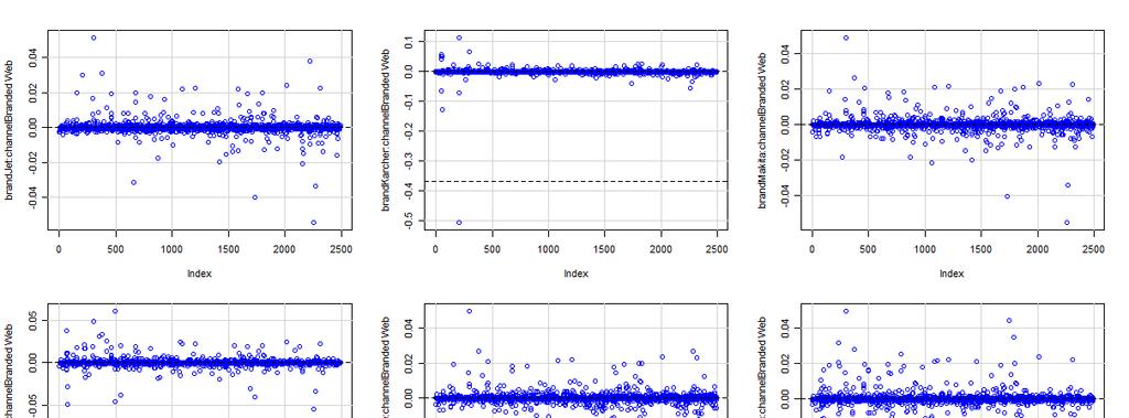
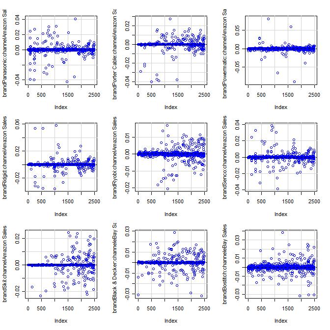
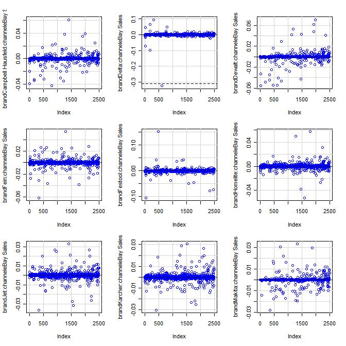
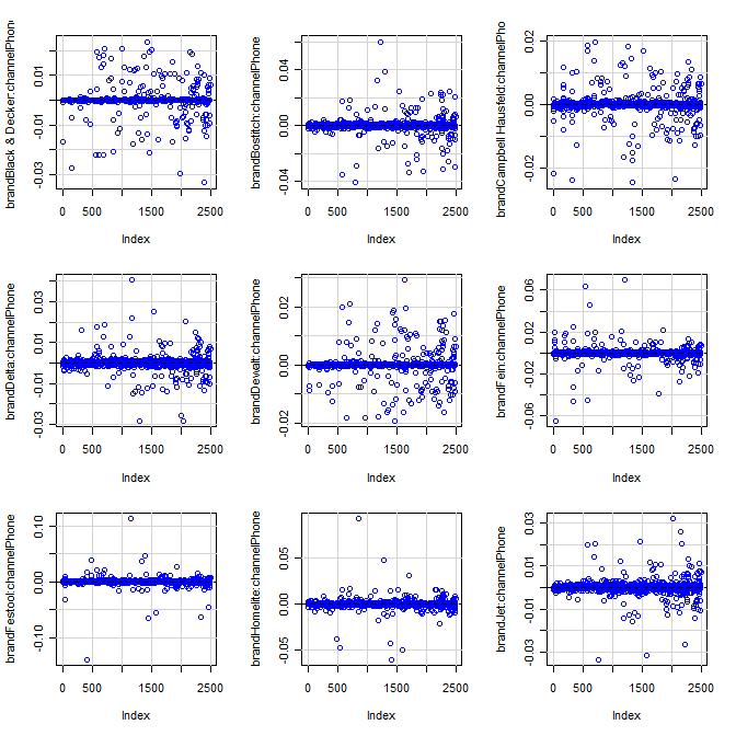
32 1-B.4: DF Beta Plots Description from the R Documentation: These functions display index plots of dfbeta (effect on coefficients of deleting each observation in turn) and dfbetas (effect on coefficients of deleting each observation in turn, standardized by a deleted estimate of the coefficient standard error). In the plot of dfbeta, horizontal lines are drawn at 0 and +/- one standard error; in the plot of dfbetas, horizontal lines are drawn and 0 and +/ P age

33 32 P age

34 33 P age

35 34 P age

36 35 P age

37 36 P age

38 37 P age

39 Appendix 1 C: glm.poisson.disp 1-C.1: Residual Diagnostics 38 P age

40 1-C.2: Univariate standardized deviance residual boxplots (Sex, Income, and Brand) Deviance Residuals Deviance Residual Deviance Residual Male Female Not Known SEX Middle High Low INCOME Bosch Black & Decker Bostitch Campbell Hausfeld Delta Dewalt Fein Festool Homelite BRAND Jet Karcher Makita Metabo Milwaukee Panasonic Porter Cable Powermatic Ridgid Ryobi Senco Skil 39 P age

41 1-C.3: Univariate standardized deviance residual boxplots (Channel, Cordless, and Condition) Deviance Residual Deviance Residual Deviance Residuals Branded Web agg_channel Amazon Sales ebay Sales Phone CHANNEL Cordless Not Cordless New Reconditioned CORDLESS CONDITION 40 P age

42 1-C.4: DF Beta Plots 41 P age

43 42 P age

44 43 P age

45 44 P age

46 45 P age

47 46 P age

48 47 P age

49 48 P age

50 49 P age

51 50 P age

52 51 P age

53 52 P age