Structural Analysis and Regional Differences in Malaysian Economy: An Input-Output Approach

Transcription

1 Structural Analysis and Regional Differences in Malaysian Economy: An Input-Output Approach March 2014 Graduate School of Social System Studies The University of Kitakyushu PhD. Dissertation Abdul Razak Bin Mohamad Dewa

2 ABSTRACT Malaysia has shown a tremendous economic growth in the Southeast Asia. Since its independence from the United Kingdom in 1957, Malaysia has gained significant achievement in economic development that transpired through the remarkable growth rate from 1966 to Malaysia had recorded an average growth of real Gross Domestic Product (GDP) of 6.7% per annum over the period from 1966 to During this period, the Malaysian economy underwent a number of structural changes, mainly caused by the reorientation of industrialization strategies as well as by variation in the composition of domestic demand. In addition, during these periods, the economy had been transformed from agriculture to manufacturing-based economy that heavily relied on manufacturing products for exports. This study focuses on the differences that arose across the regions by employing structural analysis based on Input-Output approach. The Input-Output approach is used due to its wealth of details on the structure of interindustry interactions. The input-output table provides the basis for analysis. It might be ascribable to the fact that can well measure the mutual relationship among different industrial sectors as well as different regions, quantitatively. The essence of input-output model and linkages analysis is able to identify and quantify the key sectors and spillover effects to the other sectors or regions which are important for even distribution of economic i

3 growth. The significance of any sector in an economy can be investigated by examining the interdependency in production structures. In an economy, sectors that can generate larger backward linkages and forward linkages are considered important to generate economic growth, because they can generate growth in other input supplying sectors. The linkages analysis approach is used to identify the structure of the Malaysian economy which is manufacturing oriented. The study has two objectives; first objective is to examine the viscosity of manufacturing sector as a main contribution to the sustainable of economic growth. The second objective is to examine which economic activity is the engine of growth in each region in Malaysia. The main contribution of this study is the construction of multiregional input-output tables (MRIOT), in place of national input-output tables. This is because a multiregional input-output model includes the details of transactions (trades) among sectors in each region and it will enable to investigate how a sector in one region is connected to different sector in another region. The MRIO model is also able to estimate the spillover effects and quantify impact of any funds channeled in terms of output, value added or employment in the regions originally allocated as well as the rest of the regions. Thus, it can be one of powerful tools to trace regional differences and to derive sound regional policy recommendations by addressing according to the uniqueness of each region s economic structure. In summary, the study found that the linkages analysis revealed that, manufacturing and services sectors are the key sectors for Malaysia and ii

4 act as a significant contributor for the economic growth. It was also identified that each region has a different key sector to gain maximum returns by accelerating development in those key sectors. This study indicated that the key sectors for Northern and Central regions are manufacturing and service sectors. Meanwhile, Southern region s key sector is the service sector and the key sector for Sabah region is the agriculture sector. Eastern and Sarawak regions do not have any key sectors but results showed that all sectors in Sarawak region have strong backward and forward linkages. Agriculture and service specific sectors in Eastern region have a potential to be developed as a key sector because these sectors show strong backward and forward linkages. The analysis methods used are consistent to each other because both Chenery-Watanabe and Rasmussen methods revealed the similar results with different values. Key words: Input-Output Approach, Structural Analysis, Regional Differences iii

5 マレーシアの経済構造と地域間格差の分析 産業連関分析の手法を用いた一考察 アブダルラザクビンモハマドデワ (2007D10016) 北九州市立大学大学院社会システム研究科博士後期課程 2013 年 11 月 15 日 論文要旨 マレーシアは東南アジアで急速に経済発展を遂げている国の1つである 1957 年に英国から独立後 マレーシアは経済発展に顕著な成果を遂げ 特に1996 年から2007 年の著しい成長はその代表的なものである マレーシアの国内総生産は1996 年から2007 年まで平均 6.7% の成長を成し遂げた この期間 マレーシアの経済は多くの構造的変化を経てきたが それは取り分け多様な国内の需要構造の変化と工業化への再認識の戦略によるもであった それに加え この時期に国の主要生産物は農業から製造業へ移行し 特に輸出向けの工業製品へ大きく依存してきた 本論文は産業連関分析に基づく構造分析を用いて マレーシア国内の地域に生じた様々な差異に焦点を当てた 産業連関分析の手法を用いたのは 産業間の相互作用の構造を最も顕著に表すことができると考えられるためである 特に前方および後方連鎖分析は 産業間の繋がりの方向と強さを示す指標を導出することが可能であり それらの時間的な変異を観察することにより 産業構造がどのように変化していったかを読み解くことができると考えられる 本論文の目的は以下の二つである : 第一は 産業連関分析を用いた製造部門の経済成長への貢献度合いの分析 ; 第二は 各地域における経済構造の変化と成長要因部門の特定である 本論の主たる貢献はマレーシアの多地域間産業連関表 (MRIOT) の推計とそれを用いた地域間産業構造の分析である そして その結果からある地域の一つの部門が 別の地域の異なった分野とどのように関連付けられていることを調べることが可能となる さらに 地域の差異を追跡し 各地域の経済構造の特殊性を提示しそれに応じた政策提言をおこなうことにより 健全な地域政策を得る強力な道具の一つとなり得る 以上の分析を通して マレーシアにとって製造業とサービス業が重要な分野であり 国家の経済成長に有意義な貢献として作用すべきであることが判明した 更に 各地域は異なる重要な役割を担い これらの重要な部門で各地域が発展を加速することにより 総体としての国家経済に最大限の貢献することを明示した また iv

6 地域間分析の結果は 北部と中央地域の重要な分野が製造業とサービス業であることを示した 他方 南部地域の重要な分野はサービス業であり サハラ地域では農業である 東部地域とサラワクには特別な重要分野はないが 結果的にはサラワク地域では全ての分野に 強力な低成長産業と高度成長産業の分野が存在する 東部地域の農業とサービス業分野は重要であり 発展する可能性を秘めている これらが低成長産業と高度成長産業の関連性を示しているためである v

7 ACKNOWLEDGEMENT First and foremost I would like to express my sincere gratitude and appreciations to my supervisors, Professor Dr. Takeo Ihara and Professor Dr. Yasuhide Okuyama who have provided continuous constructive comments and suggestions for improvement in completing this dissertation. My heartfelt sincere thanks to Professor Dr. Hiroshi Sakamoto, Professor Dr. Hidehiko Tanimura, Professor Dr. Keiko Tamura, and Professor Dr. Eric D. Ramstetter for their assistance, moral support, and motivation throughout this dissertation. Last but not least, it is my pleasure to thank my colleagues and friends. I am very grateful for everything they did for me and I knew they always accompany along my journey to make this dissertation possible. I deeply indebted to everyone around me and May God bless them. vi

8 TABLE OF CONTENTS Page ABSTRACT ABSTRACT (JAPANESE) ACKNOWLEDGEMENT i iv vi LIST OF ABBREVIATIONS x LIST OF FIGURES xi LIST OF TABLES xii LIST OF APPENDICES xiv I INTRODUCTION 1.1 Introduction Background of the Study Research Problems and Objectives Significance and Contribution of the Study Organization of the Study 7 II AN OVERVIEW OF MALAYSIAN ECONOMY 2.1 Introduction Historical Background The British Reign and Regional Differences Evolution of National Development Policy Regional Development Goals The Establishment of Economic Corridors Growth Trends of the Malaysian Economy Consequences of the Policies Trends in Employment Regional Development and Characteristics Territory and Population GRP and GRP per Capita Urbanization Labor Force, Employment and Unemployment Summary and Issues 44 III STRUCTURAL ANALYSIS AND REGIONAL DIFFERENCES 3.1 Introduction Concept of Input-Output Framework Demand-Driven Model 48 vii

9 IV V VI Supply-Driven Model Structural Analysis Review of Previous Studies Using Structural 53 Analysis 3.4 Methodologies for Structural Analysis Linkage Analysis: Chenery-Watanabe Method Backward Linkages Forward Linkages Linkage Analysis: Rasmussen Method Backward Linkages Forward Linkages Identification of Key Sectors Summary 66 STRUCTURAL ANALYSIS OF THE MALAYSIAN ECONOMY 4.1 Introduction Results and Analysis Chenery-Watanabe Method(Direct Linkage) Rasmussen Method (Direct and Indirect Linkage) Analysis Based on Five Aggregated Sectors Chenery-Watanabe Method (Direct Linkage) Rasmussen Method (Direct and Indirect Linkage) Summary 81 CONSTRUCTION OF MULTIREGIONAL INPUT-OUTPUT TABLE 5.1 Introduction Methods to Construct the Multiregional Input-Output Table Framework of Multiregional Input-Output Table Data Sources Construction of Multiregional Input-Output Table Location Quotients Technique RAS Technique Test the RAS Procedure 105 ANALYSIS OF REGIONAL DIFFERENCES 6.1 Introduction Verification of Estimated MRIO Table 106 viii

10 VII Verification by Intermediate Input Verification by Intermediate Demand Verification by Value Added Verification by Total Output Linkages Analysis Share of Sectors in Region Share of Sector in Final Demand Share of Sector in Value Added Chenery-Watanabe Method (Direct Effect) Analysis of Direct Backward Linkages Analysis of Forward Linkages Rasmussen Method (Direct and Indirect Effect) Analysis of Backward Linkages (Power 125 of Dispersion Index) Analysis of Forward Linkages 127 (Sensitivity Dispersion Index) 6.4 Conclusion 128 CONCLUSION AND POLICY RECOMMENDATIONS 7.1 Introduction Summary of the Study Policy Recommendations National Level Regional Level Research Limitation and Future Research 142 ix

11 LIST OF ABBREVIATIONS ECER East Coast Economic Region ECERDC East Coast Economic Region Development Council EOI Export-Oriented Industrialization IM Iskandar Malaysia IMP1 First Industrial Master Plan IMP2 Second Industrial Master Plan IRDA Iskandar Regional Development Authority ISI MDC MIDA MITI Import-Substitution Industrialization Multimedia Development Corporation Malaysia Industrial Development Authority Ministry of International Trade and Industry MP Malaysia Plan MRIOT MSC Multiregional Input-Out Table Multimedia Super Corridor NCER Northern Corridor Economic Region NDP National Development Policy NEP New Economic Policy OPP1 First Outline Perspective Plan, OPP2 Second Outline Perspective Plan, OPP3 Third Outline Perspective Plan, ODA PEMANDU Official Development Assistance Performance Management Delivery Unit RECODA Regional Corridor Development Authority SDC Sabah Development Corridor SCORE Sarawak Corridor of Renewable Energy SEDIA Sabah Economic Development and Investment Authority x

12 LIST OF FIGURES Page Figure 2.1 Map of Malaysia 9 Figure 2.2 Development Planning in Malaysia 14 Figure 2.3 The Location of Five Economic Corridors 20 Figure 2.4 Malaysian Economic Growth 1966 to Figure 2.5 Economic Activities by Percentage Share of GDP 26 Figure 3.1 Framework of Input-Output Table 48 Figure 5 Layout of the Multiregional Input-Output Model for Malaysia 90 Figure 5.1 The Overview of An Aggregation of Economic Activity Into Selected Classified Sectors 91 xi

13 LIST OF TABLES Page Table 2.1 Evolution of National Development Policy Table 2.2 Malaysia: Percentage of Employment by Sector, Table 2.3 Statistical Indexes of Each Region, Table 2.4 Urbanization Rate by State, 1995, 2000 and Table 2.5 Labor Force, Employment and Unemployment by Region ( 000) 43 Table 4.1 Chenery-Watanabe Method- Top 20 Sectors Backward Linkage 72 Table 4.2 Chenery-Watanabe Method-Top 20 Sectors Forward Linkage 73 Table 4.3 Rasmussen Method-Top 20 Sectors Backward Linkages 76 Table 4.4 Rasmussen Method-Top 20 Sectors Forward Linkages 77 Table 4.5 Five Sectors Chenery-Watanabe Method 80 Table 4.6 Five Sectors -Rasmussen Method 80 Table 5.1 Classification of Activities 92 Table 5.2 Overall Image of Producing Interregional Input-Output Coefficient of Each Region 96 Table 6.0 Estimated Malaysia Multiregional Input-Output Table Table 6.2 Extracted from the MRIO Table (Table 6.0) 107 Table 6.2a Summary of Agricultural Sector Extracted from Table 6.2 for the Northern Region 108 Table 6.2b Summary of All the Regions for Agricultural Sector by Column Sum 108 Table 6.1 Aggregated National Input-Output Table Malaysia 2005 (Million) 110 Table 6.3a Northern Region 111 Table 6.3b Eastern Region 111 Table 6.3c Central Region 111 xii

14 Table 6.3d Southern Region 112 Table 6.3e Sabah Region 112 Table 6.3f Sarawak Region 112 Table 6.4 Comparison Intermediate Input Between MRIO Table and National Input-Output Table 112 Table 6.5 Partly Extracted from the Estimated MRIO Table Verification by Row 113 Table 6.5a Summary of Mining and Quarrying Sector Extracted from Table 6.5 for the Northern Region 114 Table 6.6a Northern Region 114 Table 6.6b Eastern Region 114 Table 6.6c Central Region 115 Table 6.6d Southern Region 115 Table 6.6e Sabah Region 115 Table 6.6f Sarawak Region 115 Table 6.7 Verification by Intermediate Demand: Comparison Between MRIO Table and National Input-Output Table 116 Table 6.8 Verification by Value Added 117 Table 6.9 Extracted from Table 6.0 for Verification of Total Output 118 Table 6.9a Verification by Total Output 119 Table 6.10 Share of Sectors in the Region 121 Table 6.11 Chenery-Watanabe Method: Backward and Forward Linkages 122 Table 6.12 Rasmussen Method: Backward and Forward Linkages 126 Table 6.13 Summary of Key Sector in Each Region and The Ninth Malaysia Plan 130 xiii

15 LIST OF APPENDICES Page Appendix Table 5.0 Estimation of MRIO 168 Appendix Table 5.0 Estimation of MRIO (Continue 1) 169 Appendix Table 5.0 Estimation of MRIO (Continue 2) 170 Appendix Table 5.0 Estimation of MRIO (Continue 3) 171 Appendix Table 5.0 Estimation of MRIO (Continue 4) 172 Appendix Table 5.0 Estimation of MRIO (Continue 5) 173 Appendix Table 5.0 Estimation of MRIO (Continue 6) 174 Appendix Table 5.0 Estimation of MRIO (Continue 7) 175 Appendix Table 5.0 Estimation of MRIO (Continue 8) 176 Appendix Table 5.0 Estimation of MRIO (Continue 9) 177 Appendix Table 5.0 Estimation of MRIO (Continue 10) 178 Appendix Table 5.0 Estimation of MRIO (Continue 11) 179 Appendix Table 5.0 Estimation of MRIO (Continue 12) 180 Appendix Table 5.1 Differences from Row and Column Margins at Each Step in the RAS Adjustment Procedure 181 Appendix Table 5.1 Differences from Row and Column Margins at Each Step in the RAS Adjustment Procedure (Continue 1) 182 xiv

16 Appendix Table 5.1 Differences From Row And Column Margins at Each Step in the RAS Adjustment Procedure (Continue 2) 183 Appendix Table 5.1 Differences From Row and Column Margins At Each Step in the RAS Adjustment Procedure (Continue 3) 184 Appendix Table 5.2 Elements in the Diagonal Matrices k rˆ For k=1.., Appendix Table 5.2 Elements in the Diagonal Matrices k ŝ For k=1.., 70 (Continue) 186 Appendix Table 5.3 Aggregation of Economic Activity into Selected Classified Sectors 187 xv

17 CHAPTER 1 INTRODUCTION 1.1 Introduction Malaysia is one of the fastest growing economies in the Southeast Asian region, where from 1970 to 2005 the real gross domestic product (GDP) grew at an average rate of 6.6% (WDI, 2007). This remarkable growth might be contributed to the fast evolution of industrial sector which is able to propel the country into one of the active exporters of manufacturing goods. Prior to its independence from the United Kingdom in 1957, the Malaysian economy was heavily relied upon agricultural commodity such as rubber. However, the direction gradually changed after the independence where the commodity was well diversified into other goods. Since then, the real GDP grew by an average of 6.5% per annum for forty-eight years from 1957 to In addition, it was also observed that the influx of foreign investments in the mid-1980s, especially from Japan was one of the reasons why Malaysia was able to sustain rapid growth rate. Japan became the dominant economic actor in Southeast Asia during the 1980s, largely as a result of its Official Development Assistance (ODA) to the ASEAN countries, and moreover it was strengthened by the Plaza Accord 1985 which turned the Japanese foreign direct investment to these countries including Malaysia (Naurin, 2002). As a consequence, the structure of Malaysian economy was transformed from an 1

18 agriculture-based economy, to a manufacturing-based economy. 1.2 Background of the Study The first racial riot occurred on May, between the Malays and the Chinese in Kuala Lumpur. These riots led the government to declare a state of national emergency and suspend the parliament until The government cited the riot as a turning point for the country to give more emphasis on developing the nation fair distribution of wealth by introducing more aggressive affirmative action policies. Malaysia has implemented series of development policies to avoid the racial riot in 1969 incident from repeating. Under First Outline Perspective Plan (OPP1) covering the period , four development plans were implemented within the framework of the New Economic Policy (NEP). The NEP was introduced after the riot to promote growth with equity with the objective of fostering national unity among the various races. The Second to Fifth Malaysia Plans (Five-year Plan) aimed to construct industrial estates in all states, including encouraging foreign investments by establishing Free Trade one (FT) as a correction policy for regional differences. In line with this policy, the Second Outline Perspective Plan (OPP2), covering period , was formulated based on the National Development Policy (NDP). The NDP continued to accelerate the process of eradicating poverty and restructuring society and economic imbalances achieved by OPP1. The Outline Perspective Plan (OPP3) covering period was launched with its focus on building a resilient and 2

19 competitive nation and embodying the National Vision Policy (NVP). OPP3 also refers to the balanced regional development in the scope of building a united and equitable society. Malaysia has successfully developed from an agriculture-based economy to one focused on manufacturing, where the latter sector s value added contribution to GDP stood at 31.5% in 2005 and 80.5% share to total exports (Malaysia, 2006). However, agriculture remains the basis of livelihood for about 20% of Malaysians and contributes about 8.2% of GDP in 2005 (Malaysia, 2006). Malaysia is highly open economy and a leading exporter of electrical appliances, electronics parts and component, palm oil, and natural gas. The top three export partners are the USA, Singapore, and Japan. The top three import partners are Japan, the United States of America (USA), and Singapore (Economic Report 2006/2007). Today, Malaysia is a broad-based and diversified economy. It is the 19th largest trading nation in the world, with trade in excess of RM 1 trillion. At the same time, per capita income has increased 26 times to RM 20,841 and the incidence of poverty has been reduced to less than 6.0% (Economic Report 2007/2008). In spite of continuing economic and political stability, Malaysian government committed to restructure the society in order to rectify the imbalance income distribution, employment, ownership and control the wealth equitably distributed among the races, economic activities, and subsequently between states and regions. These were the factors that led to the racial riot on May 13, 1969 and further explained in the chapter two. 3

20 The aim of the government is to build and sustain harmonious Malaysian nation besides to continue the structural transformation towards becoming a developed nation by year Even though the economic growth contributes a lot of benefits to the development and growth of the country, it also contributes to the widening of differences among the regions in term of GDP per capita, income or employment opportunities among the races especially in the multi-racial country like Malaysia. In other words, the growth is unevenly endured across the regions; the problem of regional differences has not been improved. Political stability is the main contribution to the Malaysian economic growth and development. It is crucial for multi-racial and multi-ethnics country such as Malaysia to maintain peace and social harmony through equitably distributable national wealth regardless of races, states, and regions. Thus, this study focuses on what is the regions key sector are in order to accelerate the regional economic growth based on input-output approach. Through the linkage analysis in this study, the government is able to identify the uniqueness of each region s economic structure and hence, regional economic policies can be addressed accordingly. The most important is that each region has different characteristics that provide different economic opportunities to offer. 4

21 1.3 Research Questions and Objectives Although series of development policies have been implemented, and Malaysia is one of Southeast Asian countries experienced extremely high economic growth rates as reported in the East Asian development in 1993 by the World Bank (Page, 1994), rapid growth did not occur in all regions. The existence of regional differences affects the process of economic development. The Malaysian economy is characterized by unequal distribution of resource endowments, imperfect mobility and imbalance in infrastructure supply and an equal growth profile of regions leading to an uneven regional growth in Malaysia. The rich states experienced a higher degree of convergence rather than the poor states. The manufacturing sectors were the main economic activities especially in more developed states and able to reduce the differences between the states and regions (Hassan, 2004). Based on this backdrop, this study applied an input-output approach because the input-output table provides a snapshot of interindustry relationships in very a simple way. The objectives of this study are as follows: 1. To examine the viscosity of manufacturing sectors as main contribution to the sustainable economic growth. 2. To examine which economic activity is the engine of growth and shape regional structure in each region of Malaysia. In order to achieve these objectives, structural analysis has been employed. Linkage analysis is appropriate to be used to identify the key sectors as potential indicator to achieve more economic growth in an 5

22 economy. However, to achieve the second objective, the construction of a multiregional input-output model is needed. By doing so, the linkage analysis to identify the key sector of each region can be examined. 1.4 Significance and Contribution of the Study. The essence of this study can be seen by three aspects; firstly, the multiregional input-output model (MRIO) can be seen as an additional tool used to estimate the economic impact of the Malaysia structural changes. Structural changes can be defined as temporal changes in interactions among economic sectors (Jackson et al. 1990). Therefore, a MRIO model is able to examine the effectiveness of regional policies implementation by measuring the interregional effect due to any structural changes. Another reason is it provides regional road map because each region has different characteristics that provide different economic opportunities (Panggabean, 2004). The identification of key sectors must be sufficiently detailed and portrays interdependence among sectors in an economy. By having this regional road map, regional policies can be addressed in accordance to the uniqueness of each region s economic structure more effectively. The financial fund and investments can be channeled appropriately and wisely for the benefit of national government and other agencies to make progress in their endeavor that promise to yield the greatest return. 6

23 1.5 Organization of the Study The structure of this dissertation is divided into seven chapters. Chapter 1 provides an introduction to the study, the discussion of the basic structure and structural changes of Malaysian economy in the past decade, research problems and objectives, significance and contribution of the study. Chapter 2 highlights the background of Malaysian economy including demography, and national development policy implication. In addition, some background pertaining to the history on the colonialization prior to the independence in This provides an important information to the roots and existence of regional differences in Malaysia. Chapter 3 presents the reviews of structural analysis and regional differences. Reviews on structural analysis and methodologies are highlighted. The concept of linkages in input-output models and key sectors are explained in detail. Chapter 4 describes the structural analysis of the Malaysian economy. The Chenery-Watanabe and Rasmussen methods, normalized and weighted for both backward and forward linkages were applied on national input-output tables to identify the key sectors. The results and analysis are discussed in this chapter. Chapter 5 represents the core of this study. It attempts on methods to construct the multiregional input-output (MRIO) model. It presents three approaches; survey, non-survey and hybrid that can be used to construct the multiregional input-output model. The non-survey approach was chosen to be used to construct the MRIO table and the steps were illustrated in this chapter. 7

24 Chapter 6 presents several ways of verification of the estimated MRIO and the results are compared with the national input-output table. The analysis of regional differences was done on the estimated multiregional input-output table. The key sector in each region has been identified. Finally, chapter 7 provides summary of the research study, policy recommendations for national and regional levels, research limitations and future research and conclusions. 8

25 CHAPTER 2 AN OVERVIEW OF MALAYSIAN ECONOMY 2.1 Introduction Malaysia is located in Southeast Asia among Thailand to the north, Singapore to the south, and Indonesia to the southwest, across the Strait of Malacca. Malaysia is divided geographically into two parts Peninsular (West Malaysia) and Borneo (East Malaysia), where the East Malaysia is separated from the Peninsular by 650 kilometer of the South China Sea. Figure 2.1: Map of Malaysia Source: Department of Survey and Mapping Malaysia East Malaysia, which occupies roughly the northern part of the large island of Borneo and shares a land boundary with Kalimantan to the south, comprises of two states, Sabah and Sarawak, and one Federal Territory of 9

26 Labuan. Peninsular Malaysia, which has a landmass of 132,750 square kilometer, consists of the eleven states, namely, Johor, Kedah, Kelantan, Melaka, Negeri Sembilan, Pahang, Perak, Perlis, Penang, Selangor, and Terengganu, and two Federal Territories of Kuala Lumpur and Putrajaya. The Malaysia s population was 28.3 million at the census Malaysian population comprises of three main ethnic groups, Malays (62%), Chinese (27%), and Indians (7.6%). Out of these, 76.5 % of Malaysians live in Peninsular Malaysia and 23.5 % of them live in the East Malaysia. Malaysian population has grown at a rate of 2.6 % per annum from 2000 to 2007 (Economic Planning Unit, Malaysia). In 2006, GDP at 2000 price was Ringgit Malaysia (RM) 5.9 billion or USD1.6 billion, while GDP per capita was RM20,841 or USD5,681 (Central Bank of Malaysia Report, 2007). Section 2.2 illustrates a presentation of the historical background of the Malaysian regional economies in relation to differences among races and regions. Then, section 2.3 discusses the evolution of national development policy including regional development goals. Section 2.4 covers an overview of Malaysian economy. Section 2.5 presents the regional development and characteristics and this chapter ends with section 2.6 with summary and issues. 2.2 Historical background The purpose of this section is to explain the structure of socio-economic and demographic changes and its disparities in Malaysia, which were inherited from the colonial period, due to the colonial exploitation policies and international migration to Malaysia (Hassan, 2004). The strategic location in Southeast Asia has turned Malaysia to be a center of diversities in terms of trade, foreign influences, and colonialism. Peninsular Malaysia had undergone several phases of colonialization since The Portuguese were the first European power to establish themselves in Malaysia, by capturing Malacca in 1511, followed by Dutch 10

27 in 1641 until The Anglo-Dutch Treaty of made the British hegemony in Malaya (before having the name of Malaysia). The next phase of foreign influence was the immigration of Chinese and Indian workers to meet the needs of the colonial economy created by the British in the Malay Peninsular and Borneo. Then, Japanese invasion during the World War II ( ) ended the British domination in Malaysia before British regained the control in The British Reign and Regional Differences The presence of colonialism, which started on the west coast of peninsular Malaysia, marked a major turning point in the Malaysian history. The colonialization took place in Malacca (1785), Penang (1786), and Singapore (1824) 2 where all these states are located on the west coast. In 1826, the British formed the Colony of the Straits Settlement 3, which consisted of Penang, Singapore and Melaka and became the crown colony in 1867 while the majority of their populations were Chinese. The treaties which required the Malay rulers to appoint advisers to control all administrative matters, except those relating to Islam and the Malay customs, made the British influence in the Malay Archipelago 4 powerful. By 1800 s, the British gradually consolidated their control over the 1 This, also known as the Treaty of London (one of several), was a treaty signed between the United Kingdom and the United Kingdom of the Netherlands in London on 17 March In 1881 Singapore attained the status of a major port and commercial centre in Southeast Asia (Chee, 1983) 3 The Straits Settlements were a group of British territories located in Southeast Asia.Originally established in 1826 as part of the territories controlled by the British East India Company, the Straits Settlements came under direct British control as a crown colony on April 1, The colony was dissolved as part of the British reorganization of its South-East Asian dependencies following the end of the Second World War. The Straits Settlements consisted of the individual settlements of Malacca, Penang(also known as Prince of Wales Island), an Singapore, as well as (from 1907) Labuan. With the exception of Singapore, these territories now form a part of Malaysia. 4 The Malay Archipelago and Maritime Southeast Asia are names given to the archipelago located between mainland Southern Eastern Asia (Indochina) and Australia. Located between the Indian and Pacific Oceans, the group of 20,000 islands is the world's largest archipelago by area. It includes the countries of Indonesia, Philippines, Singapore, Brunei, Malaysia, East Timor, and most of Papua New Guinea. 11

28 Malay Peninsular, Sabah and Sarawak. In 1874, the British started direct intervention and the control of the Malay states, starting with Perak before they extended their rule in Selangor, Negeri Sembilan and Pahang. All of these states are located on the east coast, except Pahang. During this time, the disparity of income between the west and the east peninsular Malaysia had become more obvious (Hassan, 2004). By 1910, the pattern of British rule in the Malay lands was established controlling every aspect of the Malaysian life, from education to political. States in Malaya were divided into two groups: Federal Malay and Unfederated Malay States 5, and became British colonies. Federal Malay States consisted of Perak, Selangor, Negeri Sembilan and Pahang. On the other hand, Unfederated Malay States, consisted of Johore, Kedah, Kelantan, Perlis and Terengganu. Perak, Selangor and Negeri Sembilan were rich with natural resources, such as tin and rubber that encouraged British to control the Malay states. Infrastructures were constructed in these states to extract and channel the natural resources for export. Rubber then became Malaya s main export due to the booming demand from the European industries, followed by palm oil. Since these productions required a large labor force, British imported plantation workers from the Southern India and mining workers from the southern China. The percentage of the Malays (including other Malaysians) was only 32 % and 41% in the Strait Settlement and the Federated Malay States, respectively, while the balance was from the immigrant group. In the Unfederated Malay States, on the other hand, the percentage of the Malays was 84% (Hassan, 2004) The Federal Malay States, where the majority was populated with immigrant groups, changed their industrial structure from traditional agriculture to commercial sector and became the main supplier for tin and rubber to the world since the early twentieth century. These changes 5 Unfederated Malay States were protected states by British in the Malay peninsular in the first half of the twentieth century. These states lacked common institutions, and did not form a single state in international law. 12

29 created imbalance in terms of demographic pattern, economic activities, and income level among regions. The states that had less immigrant labors especially in the Malay-majority states were left behind and still dominated by the traditional agricultural sector. The creation of a multi-ethnic society in Malaysia and the role played by the various ethnic groups were deeply rooted during the British colonial period ( ). The economic heritage from the colonial times resulted in the marked segregation based on ethnicity in terms of geographical location, economic activity and political participation. Since its independence in 1957, the Malays have held most of the political arena, while other races have controlled the economic power. This political-economic dichotomy has been further enhanced by the stark regional differences, with the majority of the Malays reside in rural areas, whereas the Chinese and the Indians occupy the urban areas. 2.3 Evolution of National Development Policy Between 1950 and 2010, Malaysia has released twelve national economic plans (also known as five year economic plan) and implemented three outline perspective plans (or long-term development plan): First, Second and Third Outline Perspective plans (OPP1, OPP2 and OPP3), respectively as shown in figure 2.2 and table 2.1. Since achieving its independence in 1957 and prior to 1970, laissez-faire policy had been implemented for mainly aiming to promote economic growth with a strong emphasis on export, but not on distributional aspect. During this period, although the national economy grew rapidly at 6.0% per annum (Economic Planning Unit, 2004), the socio-economic imbalances among the ethnic groups had increased, leading to the racial riot in

30 Figure 2.2: Development Planning In Malaysia Source: Economic planning Unit, Malaysia, retrieved on Jan, 2010 available at 14

31 The racial riot exposed the inherent dangers in the Malaysia s multi-racial society, when ethnic prejudices were exacerbated by the economic disparities. Consequently, in 1971 the first long-term development plan, OPP1, was launched. It involved four sets of Malaysia plan from 1971 to 1990 with focus on eradicating poverty and restructuring society. These development plans were implemented within the framework of the New Economic Policy (NEP). Subsequently, OPP2 was launched as the successor to the NEP under the framework of National Development Policy (NDP). The NDP s aim was to sustain the growth momentum and to enable Malaysia to become a fully-developed nation by the year The sixth and seventh Malaysia Plans ( ) in table 2.1 are called for an average annual growth rate of 7.5%. The main policy of development plans in this period was toward privatization by transferring the activities and functions of public sector to private sector, encouraging the spread of industries throughout the country, increasing manufacturing in the free trade zones, and providing finance for industry through the establishment of specialized financial institutions. The OPP3 6 ( ) was launched with its focus on building a resilient and competitive nation and on embodying the National Vision Policy 7 (NVP). OPP3 emphasized on the diversification of industry and services sectors in lagged areas especially the Eastern states, Sabah, and Sarawak regions due to their agricultural based economy. The target of development plans was on creating a knowledge-based economy. The acquisition, utilization and dissemination of knowledge were considered as the basis for growth. The development of a knowledge-based economy 6 The Third Outline Perspective Plan was presented by former Prime Minister, The Hon. Dato Seri Dr. Mahathir Bin Mohamad on 3 April 2001 and the Eighth Malaysian Plan on 23 April The National Vision Policy (NVP) aims to establish a united, progressive and prosperous Malaysia nation. It endeavors to build a resilient and competitive nation, and equitable society to narrow down the social, economic and regional imbalances. 15

32 involved enhancing the value-added for all production activities through the utilization of knowledge and creating new knowledge intensive industries. The aim of this development plan was to make Malaysia more competitive with developed countries through increase in opportunities such as better access to technology for global trade and investments. The combination of increased use of knowledge and better skilled workforce could contribute towards the improving the productivity levels. 16

33 Table 2.1 : Evolution of National Development Policy Long-term Development Plan Years Five year Development Plan Plan Focus The laissez faire policy was adopted First Outline Perspective Plan (OPP1)/New Economic Policy ( ) Draft Development Plan, Malaya Emphasis on economic and First Malaya Plan rural development aimed at Second Malaya Plan promoting growth with First Malaysia Plan strong on export market Second Malaysia Plan Third Malaysia Plan Fourth Malaysia Plan Fifth Malaysia Plan Emphasis on eradicating poverty and restructuring society Second Outline Perspective Plan (OPP2)/National Development Policy, NDP ( ) Sixth Malaysia Plan Seventh Malaysia Plan Emphasis on the privatization Third Outline Perspective Plan (OPP3)/National Vision Policy, NVP ( ) Sources: Author's illustration Eighth Malaysia Plan Emphasis on knowledge Ninth Malaysia Plan -based society 17

34 2.3.1 Regional Development Goal The goal of regional development strategy under the New Economic Policy (NEP) was on regional balance and integration among the less developed states and regions in Malaysia. National government s efforts aimed at improving opportunities for social and economic advancement in the less developed states and facilitating the mobility of people across regions and creating employments. These efforts were aimed at creating a nation where all regions can share in the benefits of development and ultimately achieve the national unity. In order to promote smoothly the process of narrow down the regional differences, Malaysian government has divided the states into six regions. A region may comprise an entire state or a group of states. Thus, states in Malaysia are being composed of six regions, Northern, Eastern, Central, Southern, Sabah and Sarawak regions. The Northern Region consists of four states, Kedah, Perak, Perlis and Pulau Pinang with Georgetown as the growth center 8 ; The Eastern Region consists of three states, Kelantan, Pahang, and Terengganu with Kuantan as growth center; The Central region consists of four states, Federal Territory of Kuala Lumpur, Melaka, Negeri Sembilan, and Selangor with Kuala Lumpur as the growth center; The Southern region consists of one state which is Johor with Johor Baharu as the growth Centre; Sabah and Sarawak regions with Kota 8 Growth center acted as a catalyst growth for the secondary urban centers within their respective regions. It played an important role in urbanizing their respective regions. 18

35 Kinabalu and Kuching as the growth centers, respectively. In addition, the states in Malaysia have been divided into two categories, developed states (DS) and less developed states (LDS) by using the composite development index 9, and it is implemented from 2001 (Hassan, 2004). The developed states consist of Johor, Melaka, Negeri Sembilan, Perak, Pulau Pinang, Selangor, Federal Territory Kuala Lumpur, Federal Territory Labuan, and Federal Territory Putrajaya, whereas, the less developed states consist of Perlis, Kedah, Kelantan, Terengganu, Pahang, Sarawak, and Sabah. At the same time, the states in Malaysia were categorized into three high-income states, middle-income states and low-income states. The high-income states achieved GDP per capita almost double of the national average and an overall high rate of economic activity. On the other hand, the middle-income states achieved relatively high per capita income and the low-income states received per capita GDP less than half the national average (Malaysia, 1981) The Establishment of Economic Corridors Figure 2.4 shows the location of the five corridors in Malaysia. The Malaysian government had launched five economic corridors during the ninth Malaysia Plan (see table 6.13); Iskandar Malaysia (IM) for the Southern region, East Coast Economic Region (ECER) for the Eastern 9 The composite development index comprises of ten indicators; GDP per capita, unemployment rate, urbanization rate, registration of car and motorcycle per 1,000 of population, poverty rate, population provided with piped water, population provided with electricity, infant mortality rate and number of doctors per 10,000 of population. 19

36 region, Northern Corridor Economic Region (NCER) for the Northern region, Sarawak Corridor of Renewable Energy (SCORE) for Sarawak region, and Sabah Development Corridor (SDC) for Sabah region. Figure 2.3: The Location of Five Economic Corridors Source: The Malaysian government had spent RM244.3 billion (US81 billion.) for the development of these corridors. The development of these corridors will reduce the regional imbalance and to encourage equitable growth, investment and employment opportunities to all regions in Malaysia (Mid-term Review Ninth Malaysia Plan, 2008). The main aim of these corridors is to maximize the region's economic potential activities growth through the increasing of value added of the existing industries. Besides, to allow the nation s economic development to be balanced by shifting away from highly concentrated developed region such as the Central region and to the less developed region to grow. The five regional cities and corridors will help to propel the Malaysia s economic growth. Hence, this will close 20

37 the development and income gap between the different regions in Malaysia. The implementation of transformation programs of these corridors are jointly lead by the Performance Management and Delivery Unit (PEMANDU) and the respective authorities; Northern Corridor Implementation Authority (NCIA) for NCER. Iskandar Regional Development Authority (IRDA) for IM, East Coast Economic Region Development Council (ECERDC) for ECER, Regional Corridor Development Authority (RECODA) for SCORE, and Sabah Economic Development and Investment Authoriy (SEDIA) for SDC. 2.4 Growth Trends of the Malaysian Economy The purpose of this section is to give an overview of the Malaysian economic trends from 1966 to 2007 as shown in figure 2.3 below. The Malaysian economy had enjoyed high economic growth rate for more than four decades with its strong growth momentum at an average of 6.71 % per annum even though facing several crises during this period. Four major crises have been identified during the observed period: oil crisis of , commodity/electronic crisis of , Asian currency crisis of , and US financial crisis in The oil crisis was originated from the Organization of Petroleum Exporting Countries (OPEC) which had reduced the production of oil and placed the embargo on the nations that support for Israel such as America and Western countries. OPEC raised the price of crude oil and led to global recession including Malaysia. However, Malaysia was not seriously affected since crude oil 21

38 constituted about 4% of total exports. Although the volume of crude oil exports declined, earnings from oil exports recorded increase of 22.7% compared to This was supported by the increased earnings boosted from the mining sector, which contributed to 16.4% of total gross exports in In addition, demand for Malaysia s agricultural commodities rose by 73.3% compared to The strong performance from other sectors of economy and also strong private consumption and investment in 1973, had contributed to increase in real GDP by 11.7% while it was 9.4% in 1972 (Chio, 2005; Okposin and Cheng, 2000). Generally, this oil crisis benefited Malaysia in terms of strong demand for its commodity exports. Thus, Malaysia cushioned the impact of inflation of oil prices and became one of the lowest inflation rate countries in the world. Secondly, the commodity/electronic crisis lasted between1985 and 1986 with economic decline of 1.7 % in It was considered as the first recession experience for Malaysia since its independence. Malaysia s manufacturing sector is dominant on electronic and electrical-based products and contributed to the nation s growth. The global recession in 1986 had led to a weak demand for electronic and other commodity products and affected the related industries severely, particularly in the semiconductor industry, and the overall Malaysia s GDP growth (Okposin and Cheng, 2000). The manufacturing sector recorded the decline of 3.8% while national unemployment rate increased by 3.6% in 1985 national government had taken initiatives to utilize the foreign borrowings to investment programs, major structural adjustments in domestic expenditures and embarked on privatization program on services 22

39 Real GDP Growth Rate and projects; overall GNP successfully at the average deficit of 9.8% against to 14% during (Okposin and Cheng, 2000). Figure 2.4: Malaysian Economic Growth 1966 to 2007 Economic Growth 1966 to % GDP 15% 10% Oil Crisis Electronic Crisis Asian Currency Crisis USFinancial Crisis 5% 0% -5% -10% Year Sources: Economic Planning Unit, Malaysia, World Bank Indicator 2006, Asian Development Bank Database Thirdly, the Asian financial/currency crises 10 of plunged 10 According to the Asian Development Bank (ADB) report 1999, there were two economic views on the real causes of this crisis; it was caused by poor economic fundamentals and policy inconsistencies and Asia victim to a financial panic of negative sentiment prophecy. According to fundamentalists, serious structural problems, regulatory inadequacies and close links between public and private institutions caused the Asian crisis (Okposin, 2000, p.113) Specialist in Industry and Trade Economics Division, Dick K. Nanto in CRS Report for Congress, 1998 stated that the cause of this crisis was a shortage of foreign exchange. This caused the value of 23

40 Malaysia into a severe economic crisis. The economic growth in 1998 sharply declined to negative 7.4 %. The Asian financial crisis was initiated by two rounds of currency depreciation; an extreme drop in the value of the Thai baht, Malaysian ringgit, Philippine peso, and Indonesia rupiah; and downward pressures on Taiwan dollar, South Korean won, Brazilian real, Singaporean dollar and Hong Kong dollar. The crisis began in May 1997, with the attack of foreign currency speculators on Thailand s currency, Baht (Charles, 2008; Naurin, 2002; Aghevli, 1999). However, the Malaysian economy was rapidly recovered through the prudent and immediate structural adjustments and financial sector reform. Malaysia adopted an orthodox approach, such as tightened fiscal and monetary policies, which included the pegging of Malaysian ringgit to the US dollar at US$1= RM3.80 (Jomo, 2001),deferred huge infrastructure projects and cutback in government expenditure in order to curb the increase in the inflation rate. In the mid-1998, the government decided to ease its fiscal and monetary policies to prevent further contraction of the economy by allowing socioeconomic projects as ensuring the living standards, especially the poor and lower income groups not badly affected. One of the efforts to ease monetary policy was by reducing the Central Bank s intervention rate in the money market. Consequently, in 1999, the real GDP rebounded and grew to 6 %. Lastly, the US financial crisis began in Although the Malaysian currencies and equities in Thailand, Indonesia, South Korea and other Asian countries to fall dramatically. 24

41 economy seemed to be recovered from the financial crisis with GDP growth rate of 8.9 %, the growth was hindered because of the downward trend of the US economy due to the collapsed of dot-com bubble 11 in 2000 and the September 2001 terrorist attacks. The Malaysia s economic policy over-emphasized exports rather than domestic demand, and made it too dependent on foreign markets. The sharp slowdown in the U.S economy implied sluggish demand for electronic and electrical products. In the middle of 2001, sales value of manufacturing sector dropped by 11.2 %, semi-conductors and other electronic components and communication equipment was shrunk by 27.4 % (The Nautilus Institute, 2001). Then, the growth rate had bounded back to a steady growth at an average of 5 % per annum from 2002 to In terms of economic structure, the Malaysia s economic activities can be categorized into three main sectors: primary, secondary and tertiary sectors as shown in figure 2.4. Primary sector comprises of agricultural, forestry, fishing, mining and quarrying, while secondary sector comprises of manufacturing alone. The tertiary sector consists of utilities, construction, wholesales and retails, hotel and restaurants, transportation, storage and communication, finance, insurance, real estate and business services and other services. 11 A group of internet-based companies which referred as dot-coms and speculated their stock prices will shoot up if they added e prefix to their name com at the end. 25

42 Percentage of Share Figure 2.5: Economic Activities by Percentage Share of GDP Economic sector by Percentage Share of GDP 100% 90% Terti ary Secondary Pri mary 80% 70% 60% 50% 40% 30% 20% 10% 0% Sources: Economic Planning Unit, Malaysia, World Bank Indicator 2006, Asian Development Bank Database Year Prior to the independence in 1957, the economic development of Malaysia depended mainly on primary sector. In 1966, primary sector contributed 39.9 % to the national GDP and steadily declined to 14.2 % in The primary sector has become no longer effective because of the instability of agricultural commodity prices. Furthermore, this sector is unable to absorb the expected increase in labor force due to rapid population growth in the early 1960s. The First Malaysia Plan, was introduced by the national government to diversify the primary sector in order to eliminate its total dependence on rubber and tin. This was done 26

43 by adopting an import-substitution strategy as an essential part of the growth strategy. Besides, the national government diversified agriculture sector to include other commodities (Samudram, 2007; Okposin and Cheng, 2000). In the same period, secondary sector contributed % to GDP and the amount had gradually increased to 32.1 % in On the other hand, tertiary sector, contributed a significant portion and an average of 50 % to GDP throughout the period. This sector was expected to play a larger role for supporting the future growth Consequences of the Policies The structural change of the Malaysian economy occurred based on the several development policies implemented by the national government to ensure the sustainability of economic growth. Historically, when Malaya (name of Malaysia before independence) gained her independence in 1957, The Malaysian government has decided to implement industrialization policy through several stages based on the Harrod-Domar approach, where industrialization was conceived as the engine of growth (Hassan, 2004). The implementation of industrialization policies can be grouped into four phases. First phase, import-substitution industrialization (ISI) policy from 1958 to 1969; second, the export-oriented industrialization (EOI) from 1970 to 1980; third, the second round of ISI from 1981 to 1985; finally, second round of EOI from 1986 (Drabble, 2000; Alvi, 1996). During 1958 and 1969, the federal government had implemented the import-substitution industrialization (ISI) policy under the strong 27

44 implementation of primary commodity exports, such as petroleum, tin, rubber and oil palm. The policy aim was to reduce foreign dependency of a country's economy through local production of food and industrial products to more self-sufficient and less vulnerable to adverse terms of trade. This was done by implementing tariff and non-tariff protection in the domestic market through the establishment of the Tariff Advisory Board (TAB) in This policy had two main aims: to absorb the increase in labor force, which agriculture was alone unable to absorb; and to promote economic diversification for sustainable economic growth (Okposin and Cheng, 2000). A few institutions were set up such as Malayan Industrial Estates Limited and Malaysian Industrial Development Finance to promote ISI, besides provision of infrastructural facilities by setting up of industrial zones and cheap credit. However, the ISI had limitations; high import content of intermediate and capital goods leading to limited linkage effects, little technology transfer as well as low value added. Other than that, the protected industries remained inefficient and no effective appraisal to ensure these industries became globally competitive was proposed (Rasiah, 1995). Most of the protected industries were foreign owned which leading to huge leakages. ISI also failed to absorb the excess of labor force and leading to relatively high unemployment levels and thus, created the political instability. The worst part of this approach was failed to close the income gap between the ethnic Chinese, who were rich and urban and ethnic Malays, who were poor and rural. In fact, it had widened, and led to the racial riot of May 1969 (Gomez and Jomo, 1999; Alavi, 1996). 28

45 Because of ISI limitation such as high regional concentration that led to region imbalances, protected industries were largely foreign-owned which led to huge leakages, export-oriented industrialization (EOI) was adopted for ten years starting from The EOI successfully eased the social tension and secured the national unity, besides the main purpose of promoting local production for export. EOI extended larger international market compared to the limited domestic market during ISI. Government had introduced tax incentives, such Investment Incentive Act (1968), the Free Trade one Act (1971) (FT) and Licensed Manufacturing Warehouse Act (1973) (LMW) and establishment of Export Processing ones (EP) were promulgated to attract more both domestic and foreign direct investment (FDI) to establish their manufacturing plant and promote manufacturing exports. EPs have significant impact in EOI to transform the industrial sector into a significant economy activity. EPs were established to attract export-oriented multi-national companies (MNCs) to invest in Malaysia. Most of the EP and licensed manufacturing warehouses were electrical and electronics firms and textiles and garments factories. They employed low-wage labor to assemble imported raw materials and component for export. As a result, the exports of electrical and electronic products and textile and garments contributed 60% of manufactured exports within a decade of EOI implementation (Kanapathy, 2000). Malaysian economy was then, heavily dependent on manufacturing especially from electrical and electronic and textiles and garments sectors which emerged as leading manufactured exports. In addition, lack of technology transfer or skill development took place 29

46 and the backward and forward linkages between manufacturing and other sectors in the economy were weak. Most of the establishments of new industries were assembling components and less value added. The manufacturing sector was not globally competitive, productive, and efficient. The FTs and LMWs practiced bureaucratic that prevented the development of links between them and firms operating in the principle custom areas. The financial incentives were only given to the firms that had meet high levels of export and imports (Rasiah, 1995). Although EOI successfully brought down the unemployment rate by to absorbed labor surplus, but was only low wage employment. Furthermore, Malaysian economy was affected by a number of trade problems especially from the international demand on electronic and electrical export and the world recession in early 1980s, which worsened the situation. Subsequently, Malaysia s export earnings stagnated and to redress these weaknesses, government focused on a second round of ISI based on heavy industries. In 1981, Heavy Industries Corporation of Malaysia (HICOM) was established, a public sector company to lead the heavy industrialization program. The heavy industries targeted under this program included the national car project, iron and steel mills, cement factories, a petrol refining and a petrochemical project, and a pulp and paper mill. These projects needed high capital intensity, long gestation periods and economies of scale. The main objective are: a) to initiate domestic industry linkages value chain as to achieve deeper integration and higher value added; b) promote greater technological development 30

47 through research and development. To ensure the success of this policy, the Malaysian government adopted the import restriction trade policy to protect industries such as car manufacturing, steel mills and cement factories. For instance the protection rate for the iron and steel industry rose by 140%, from 28% in 1969 to 168% in 1987 (Edwards, 1990). However, these protected industries failed to perform as expected, and other problems contributed to the failure such as poor domestic linkages, the limited size of the domestic market and slow growth and failure to penetrate global market. As a result, the Malaysian government bore the heavy cost of production and most of them were funded by the public investment based on the external borrowing. The poor performance of substituting industries, due to the worldwide economic recession in 1985 and high external debt, forced the Malaysian government to restructure and privatize many of the state-owned enterprises including the heavy industries and decided to shift back to EOI policy (Jomo, 1990; Jomo and Edwards, 1993). Under this second round of the EOI policy, the government introduced a series of Industrial Master Plans (IMPs) for a period covered from 1986 to 2020 and it was divided into three phases: IMP , IMP , and IMP3, The main focus points were a renewal of export orientation and a more liberal trade regime. The reorientation of the economy, Malaysia had registered tremendous growth in the 1990s. The IMP1 s ( ) main target was to set foundation to make manufacturing as a leading sector of economy. Its main objectives: accelerated growth of manufacturing, efficient utilization of the nation s 31

48 natural resources, and development of indigenous technological capability. The promotion of resource-based industries was emphasized because it had developed a strong foundation with higher local content and the diversification of non-resource-based industries. Substantial incentives such as Promotion of Investments Act 1986 and Industrial Co-ordination Act, 1975 (ICA) to provide wider incentives for investment in manufacturing, agriculture, and tourism were granted to foreign investors to encourage investment and exports especially to those products that significant importance to the country, priority products. The scope of ICA was amended to be more relaxed to allow companies with less than RM2.5 million shareholder funds or engaging more than 74 full-time workers to operate without licenses. Previously, RM RM250,000 or 25 workers required operating licenses. The IMP1also stressed the importance of science and technology and human resource development in the industrialization process. Thus, the incentives were provided for training and for research and development to prepare workforce with industrial and technical skills. The training is important to develop indigenous skills in product design and production technology. IMP2 ( ) laid the orientation to make the manufacturing sector to be more globally competitive, productive and efficient by strengthening industrial linkages, increasing value added activities and enhancing productivity. Its two key trusts were manufacturing and industrial clusters. Manufacturing has two dimensions: expand along the value chain to include higher value added activities and strengthen the whole value chain 32

49 to raise productivity. On the other hand, cluster based industrial development was to broaden the concept of industry by way of agglomeration of related activities that comprising of industries, suppliers, supporting business services, infrastructure and institutions. The establishment of technical institutions was to provide skilled labor to ensure the plans run smoothly. There were eight clusters to be focused during the IMP2; electronic and electrical, textiles and apparel, chemicals, resource-based industries, food processing, transportation equipment, materials, and machinery and equipment. In 1996, the government launched the Multimedia Super Corridor (MSC) conceived as a super high technology park to enable the Malaysian to participate and benefit from the global information revolution. A MSC has its own advisory panel consists of experts and corporate leaders from the global community and Malaysia to provide advice (Yusof and Bhattiasali, 2008). The establishment of MSC is to recognize the gap that existed between Malaysia and other developed countries as to attract high-tech Multinationals to share their skill with Malaysian firms. For this purpose, MIDA had set up very attractive and competitive incentives. In the same year, a Multimedia Development Corporation (MDC) also established. The MDC acts as adviser to the government on MSC laws and policies, responsible to implements and monitors the MSC program, and processes the applications for MSC status. After six years the IMP2 implemented, the MSC managed to attract 50 world class companies and to make Malaysia their headquarters (Jusawalla and Taylor, 2003). Due to some other reasons including the Asian Financial Crisis early 33

50 1997 and the manufacturing sector started to loss the competitiveness due to rising of production costs and cheap exports from China, Vietnam and Least Developed Countries, the economy growth did not meet the targets as expected. The government had liberalized the economy by removed some of the restrictions impose to FDI as to accelerate the growth but it did not worked. The other alternative was the launched the IMP3 ( ) in line with the Vision 2020 where Malaysia envisaged to achieve the status of fully developed nation by It is on-going of all the efforts in IMP2 with emphasis given to strengthen on inter-cluster linkages and designed subsectors within each cluster to be more selective, for example, nano-technology and microelectronic within the electronic and electrical. The objectives of IMP3 are to achieve long-term global competitiveness through transformation and innovation of the manufacturing and services sectors. Under the IMP3, the government stress on the importance of the service sector as the engine of growth. The government has taken major improvements to induce investments, linkages, exports, training and research and development. There were 12 industries, six were non-resource based and the rest were resource based had been identified in the manufacturing sector for further development and promotion. The non-resource based are electrical and electronics; medical; textiles and apparel; machinery and equipment; metals; and transport equipment. The resource-based are petrochemicals; pharmaceuticals; wood-based; rubber-based; oil palm-based; and food processing (Alavi, 1996). The non-government services, eight sub-sectors have been identified for 34

51 greater development and promotion: business and professional services; distributive trade; construction; education and training; healthcare services; tourism services; services; and logistics (MITI, 2006). The identification of target industries was made based on their potential in growth and exports. Under this policy, it is targeted that the manufacturing sector to grow at 5.6% per annually and contribute 28.5% to GDP in 2020 and the total investments of RM412.2 billion (RM27.5 billion annually). The non-government services is expected to grow at 7.5% annually and contribute 59.7% to GDP in 2020 and total investments of RM687.7 billion (RM45.8 billion annually). It is targeted exports to increase to RM1.4 trillion and total trade to increase to RM2.8 trillion. While total factor productivity (TFP) to grow at 2.6 % annually and contribute 41.4% to GDP during the IMP3 period. More attractive incentives were given to promote or enhance economic or technology development of the country such as the extension of tax relief for a further 5 years at the end of the initial tax period of 5 years for companies that incurred expenditure of fixed assets of RM 25 million or more, or companies that employed more than 500 employees or more. Special incentives were also given to the development of small and medium enterprises (SMEs) as to accelerate the industrial linkages (Kanapathy, 2000). During the period of IMP3, the Malaysian economy is expected to grow at an average of 6.3% after taken into consideration of all the sectors were going to decline in their contribution to GDP by 2020 except services sector 35

52 (MITI, 2006). The IMP3 were outlined 10 strategic thrusts to assist the achievement of the macro targets: enhancing Malaysia s position as a major trading nation; generating investments in the targeted growth areas; integrating Malaysian companies into regional and global; ensuring industrial growth contributes toward equitable distribution and more balanced regional development; sustaining the contribution of the manufacturing sector to growth; positioning the service sector as a major source of growth; facilitating the development and application of knowledge intensive technologies; developing innovative and creative human capital; strengthening the role of private sector institutions; and lastly creating a more competitive business operating environment (MITI, 2006). Although Malaysia has been affected by the rising production costs, tightening labor market, cheap exports from China and Vietnam and 2008 world economic crisis, foreign investors still preferred Malaysia as destination for investments especially in the manufacturing sector. They continued to reinvest and expand their operation in Malaysia especially in higher value added products. FDI has recorded increased growth every year since 2003 for five consecutive years. Foreign investments in electrical and electronics industry accounted RM6.48 billion out of RM11.9 billion of diversification projects.in The foreign firms assisted in boosting the manufacturing sector in Malaysia through production of goods for export. They benefited the country through employment creation and technology transfer. With the continuation of liberalization in trade and investment, infrastructure, incentives and competent labor force, Malaysia is able to 36

53 become attractive destination for investment and benefit from their spillovers to the development of local industries Trends in Employment Since its independence, the Malaysian economy has experienced of significant structural changes, from the agricultural based economy to a manufacturing dominated economy as the source of growth. The increase of population was from 10.9 million in 1970 to 25.7 million in 2005 at a growth rate of 2.3% per annum (DOSM, 2012b; Economic Planning Unit, Malaysia) and it needed employment opportunities. Table 2.2 shows that agriculture sector was the main contributor to the national economy in 1970 and the total labor force heavily relied on this sector. However, the agriculture sector s capacity to generate new employment was declining. Meanwhile, the share of employment had gradually changed to manufacturing sector, when the government started implementing the ISI policy to diversify the economic activities, not totally dependent on agricultural sector, for sustainable economic growth. Table 2.2 Malaysia: Percentage of Employment by Sector, Sectors Agricultural, Forestry, Live-stocks & Fishing Mining & Quarrying Manufacturing Construction Transport, Storage & Communication Finance, Insurance, Real Estate & Business Services Government services Other Services Source: Economic Planning Unit, Malaysia available at Note: other services include utilities, wholesales, retails, hotel restaurants services. 37

54 Furthermore, the implementation of the second round of EOI policy became one of the reasons for the increase in per capita GDP, which promoted and broadened the manufacturing sector. Thus, labor demand for manufacturing sector has been increased at a faster rate than the increase in labor supply especially for the developed states where rapid economic growth was experienced. Consequently, the Malaysia s unemployment rate was reduced from 7.5 % in 1970 (Malaysia, 2001) to 3.2% in 2007 (DOSM, 2012a). The national government expected the manufacturing sector to play a leading role in employment generation (Malaysia, 1971; MITI, 1996). In 2007, the share of employment in manufacturing sector, increased to 29.2% with the policies promoting the export-oriented and labor-intensive industries, such as textile and electronic. In addition, Malaysia has been also rapidly urbanized, and there is an urgent need to create employment opportunities for the fast growing urban population. The employment structure is expected to undergo another notable change with the government s vision to gear country towards IT-based economy by Regional Development and Characteristics Each region has different characteristics that provide different potential capabilities for economic growth. It is important for the national government to have regional development road map. This road map is to help the policy makers to address and make better region economic policies based on the characteristics of each region s economic structure. In addition, the national government has to identify the key sectors in each 38

55 region and accelerate the development in those key sectors in order to make progress in their endeavor Territory and Population As shown in table 2.3, in terms of territory, the Sarawak region is the largest, covering 124,450 square kilometers, accounting for 38% of the country. The smallest region is the Central region which covers 16,504 square kilometers, and accounts for 5% of the total territory. With regard to population, the Central region is the most populous, with population of 8.24 million in 2005, accounting for 32% of the national population. The lowest populous region is the Sarawak region, with population of 2.30 million and, 9% of the total national population. In terms of population density, the Central region is ranked first with the density of 499 people per square kilometer; and the Sarawak region has the lowest density, at 18 people per square kilometer. 39

56 Table 2.3 Statistical Indexes of Each Region, 2005 Northern Region Eastern Region Central Region Southern Region Sabah Region Sarawak Region Malaysia Total Land Area (sq km) 32,256 63,944 16,504 18,987 73, , ,761 Total Population ('000) 5,639 3,726 8,239 3,020 3,113 2,300 26,036 Population Density Total GRP (in RM million at constant prices 2000) 79,745 40, ,017 44,276 27,395 43, ,941 GDP Per Capita (in RM million at constant prices 2000)) 14,142 10,904 22,213 14,661 8,800 19,077 89,797 Manufacturing sector: Number of establishment (%) Value Added (RM'000) 26,720,199 10,156,964 46,742,133 15,509,063 3,064,342 16,017, ,210,258 Urbanization Rate (%) Average annual growth rate (%) of urban population ( ) Source: Various Malaysia Plan and various State/District Data Bank Malaysia and author's calculation Note: 1.Population data refers to mid-year population 2. Average Annual Growth Rate of Urban Population is calculated by author from year 2000 to

57 2.5.2 GRP and GRP per capita Based on table 2.3, the Central region has the largest gross regional product (GRP), RM183 million in 2005 and accounting for 43.7% of the national figure; the Sabah region has the smallest GRP, RM27.4 million, and accounting for 3.6%. The former was 7.3 times higher than the latter. The Central region has the highest GRP per capita, RM22.2 million and is the only region surpassed the national average level; the Sabah region has the lowest rank with the GRP per capita RM8.8 million Urbanization Urbanization is defined in three ways; first, the social process whereby cities grow and societies become more urban; second, the process of the formation and growth of cities; lastly, a historical transition from being mostly rural to predominantly urban (Gantsho, 2008). A common perception can be derived based on historical trends, as documented by the United Nation and empirical studies done by Njoh (2003,) there is a positive correlation between the percentage of a country s level of urbanization and the country s income, as measured by GDP. Thus, urbanization can be considered as a fuel of economic growth. Table 2.4 Urbanization Rate by State, 1995, 2000 and 2005 REGION Urbanization Rate (%) Average Annual Growth Rate of Urban Population (%) Northern Eastern Central Southern Sabah Sarawak MALAYSIA Sources: 8th Malaysia Plan and author's calculation From table 2.4, urbanization rate in 2005 shows that the Central region has the largest urbanized population at 81.6%. This was followed by the 41

58 Southern region with 69.1% and the Northern region with 57.7%. The Eastern region, which consists of less developed state, was the lowest in terms of urbanization rate, recorded 43.6% in By looking at an average annual growth rate of urban population in table 2.4, the Sabah region recorded the highest rate in 2000, which was 7.7%. The Southern region was the second followed by the Central region. Meanwhile, the Eastern region still recorded the lowest among the regions. In 2005, Sabah region recorded the highest rate of urban population followed by Sarawak region and Southern region. There are three regions that are categorized under the region below the national average annual growth rate of urban population: Northern, Eastern, and Central regions. The Eastern region was the lowest rank among the three regions Labor Force, Employment and Unemployment Table 2.5 shows that the levels of labor force and employment from 1995 to In general, all regions had an increase in the employment level while the unemployment rate decreased. The Central region dominated the highest level of employment in 2005 and the Sarawak region recorded the lowest the in ranking. In terms of unemployment rate in 2005, the Sabah region was lagged behind in providing employment opportunities. The Sarawak region had the smallest number for labor force, with 1.1 million in 2005 compared to the Central region, 3.4 million. As for average annual growth rate for labor force and employment, the Sabah region shows the highest growth for labor force and employment, 9.4% and 9.3%, respectively in seventh Malaysia Plan ( ). While in eighth Malaysia Plan ( ), were 5.2% and 5.3%, for labor force and employment respectively. 42

59 Table 2.5 Region Labor Force, Employment and Unemployment By Region ('000) Labor force Average Annual Growth Rate (%) Employ Unemploy rate (%) Labor force Employ Unemploy rate (%) Labor force Employ Unemploy rate (%) Labor force 7MP Employ Labor force 8MP Employ Northern 1, , , , , , Eastern 1, , , , , , Central 2, , , , , , Southern , , , , Sabah , , , , Sarawak , , MALAYSIA 8, , , , , , Source: Eighth Malaysia Plan , Department of Statistics Malaysia 43

60 2.6 Summary and Issues The economic heritage from the colonial time resulted in the marked segregation based on ethnicity in terms of geographical location, economic activity and political participation. The national government has been implementing various development plans and policies with the main objectives to make equal distribution of economic growth, and to narrow the gap of socio-economic disparity among ethnic groups and across regions. It appears that these policies and plans have shown positive impact although not fully effective as discussed in this chapter. It is impossible to achieve complete regional equality due to differences in the development potential of each region and it is deeply related to the history. But, there are possible ways to improve these differences through development of regional road map (Panggabean, 2004). The purpose of regional road map is to identify and understand these local characteristics to make progress by the local government and private sectors. Malaysian economy currently relies on manufacturing sector but there exist regional differences of economic potential. There are two main objectives of the study; to examine the stability of manufacturing sectors as main contribution to the sustainable economic growth and to examine which economic activity is the engine of growth for regional economies. The second objective requires the construction of multiregional input-output table and structural analysis to identify key sectors in regional economies by applying interindustry linkages approach. 44

61 CHAPTER 3 STRUCTURAL ANALYSIS AND REGIONAL DIFFERENCES 3.1 Introduction There are several views by economists regarding the structural change of economies. According to Simon Kuznets (1956), structural change is the fall in the importance of agriculture, the rapid rise in industry and the gradual increase in the weight of services in the economy as a stylized pattern of development using historical time series data for industrialized economies. Chenery and Taylor (1968) argued that there are three patterns when structural change takes place: firstly, the share of agriculture in GDP and employment falls as economies grow richer. Secondly, the share of industry in GDP and in employment rises, but the relationship between per capita incomes and the share of industry in employment is non-linear, and lastly is the share of services in GDP and in employment rises unambiguously as economies grow richer. Chenery and Syrquin (1975, 1989) said structural change can be described as the economy grows. Structural change occurred when the production shifts from primary (agriculture, fishing, forestry, mining) to the secondary (manufacturing and construction) to the tertiary sector (services). Structural change can also be defined as temporal changes in interactions among economic sectors. Malaysia underwent structural change, when secondary sector s 45

62 production suppressed primary sector in One of the factors that contributed to the expansion of secondary sector was the implementation of export-oriented policy and foreign direct investment driven economic development (akariah and Ahmad, 1999). Kamarudin and Masron (2010) added, the Malaysian economy has undergone a number of structural changes, mainly caused by the reorientation of industrialization strategies as well as by variation in the composition of domestic demand. When the country underwent structural change, the structure of regional economy may have also changed. Thus, structural analysis can be used to examine the Fundamental Economic Structure (FES) of a nation and region using the data from input-output table. This is because each input-output table contains a number of economic activities, which collectively provides a data set for the structure of the economy. Simple techniques such as multiplier analysis, linkage and key sector analysis (Rasmussen, 1957; Hirschman, 1958) or hypothetical extraction methods (Dietzenbacher and van der Linden, 1997) are used to identify the key sector with the highest level of backward and forward linkages that plays an important role in determining the overall growth rate in the economy. For the purpose of this study, input-output analysis is used for several reasons: the major strength of input-output table is its versatility and it provides detailed information on the direct, indirect and induced effects of different industries in the given economy. Another reason is that it provides fundamental snapshot of the structure of interindustry linkages in an economy (Ihara, 2004; Loomis and Walsh, 1997; Miernyk, 1965). 46

63 This chapter is divided into six sections. Section 3.2 explains the concept of input-output framework. Section 3.3 provides a review of the previous studies on structural analysis. Section 3.4 discusses the methodologies for structural analysis. Section 3.5 is the definition of key sectors analysis used in this study and the last section 3.6 is the summary of this chapter. 3.2 Concept of Input-Output Framework Input-output analysis has become one of the most important tools in macroeconomics. The input-output table is one of the media, which provides comprehensive information on all the production activities of one s economy. The main objective of the input-output framework, developed by Leontief in the late 1930s, is to study the interdependence among the different sectors in any economy in monetary unit (Miller and Blair, 2009, 1985). There are two types of models for an economy wide interindustry model; the demand and supply driven input-output models. The demand driven input-output model is used for deriving the backward linkages, while supply driven input-output models are used for deriving the forward linkages. The reason for these dual models is to determine the input side of the sectors which purchases other sector s products (backward linkage) and the output side in which the sectors sell their own products (forward linkage) to be used in the production of the other sectors. The main differences between these two models are that the Ghosh supply-driven model uses fixed output coefficients and the sectoral outputs are calculated from exogenously specified primary factors (Rose and 47

64 Miernyk, 1989). The output coefficients are also known as sales or allocation coefficient describing the fixed part of each additional unit of output in sector i that flows to sector j. The Ghosh model assumes a fixed allocation of output over the sectors. On the other hand, the Leontief model is based on the assumption of fixed input coefficients, expressing that each additional unit of production in sector j requires the fixed amount of input over the sectors. The demand-driven model derives the sectoral outputs from exogenously specified final demands Demand-Driven Model Originally, the Leontief demand-driven model aimed to study the degree of interindustry linkages among the industries. Figure 3.1: Framework of Input-Output Table Intermediate Demand Sector j (j = 1,.,n) Final Demand Total Output Intermediate Sector i Input (i = 1,n) zij Yi Xi Primary Input Total Input Vj Xj Figure 3.1 shows the industry by industry input-output framework. For each sector, the value of total production X i is the sum of the intermediate demand z across the purchasing sectors and the final demand ij Y i and 48

65 this relationship can be represented as: X i n z j1 ij Y i (3.1) Where, X i is total output sector i z is the intermediate input of sector from i to j ij Y i is the final demand The input coefficient implies that the quantity of input required from each industry to produce one dollar s worth of a given industry s output. The input coefficient can be presented as follows: zij aij (3.2) X j Where, a is the input coefficient of from sector i to j ij z is the intermediate input from sector i to j ij X is the total input for sector j j It can be presented in the following equation form: X i a X Y (3.3) ij j i Equation (3.3) can be expressed in the following matrix from: X AX Y (3.4) Equation (3.4) can re-written as Y I AX (3.5) Or X 1 I A Y (3.6) Where, X is a vector of total output 49

66 The 1 I A A 1 Y is a vector of final demand A is the nxn matrix of input coefficient I is the nxn identity matrix, and I Is Leontif inverse or total requirements matrix is known as the Leontief inverse matrix, which shows the total production of each sector required to satisfy the final demand in the economy (Miller and Blair, 2009) Supply-Driven Model Ghosh supply-driven model was formulated by Ghosh (1958). It serves as an alternative to the Leontief demand-driven model. The elements from the Ghosh model were suggested to be more appropriate for the forward linkage measure and the row sums of the Ghosh inverse as a better measure for the total forward linkages (Miller and Blair, 2009; Adamou, 1995; Augustonovics, 1970). The output coefficient can be defined as zij bij (3.7) X i Where, b is the output coefficient of sector from i to j ij z is the intermediate input of sector from i to j ij X i is the total output of sector i The total input for industry j is the sum of intermediate demand z and ij value added (or primary input) V as follows: j 50

67 X j n z i1 ij V j (3.8) z ij is the amount sector i supplies to all sectors in the economy as inputs in their production process. By replacing the z in the equation (3.8) by ij b as in equation (3.7), we X ij i obtain the following equation: X j b X V (3.9) ij i j Matrix form of equation (3.9) is: X ' ' X B V Or can be written as X I B V (3.10) ' 1 Where, ' X is a vector of total input V is a vector of primary input. B is a nxn matrix of output coefficient, B 1 I is a nxn identity matrix I is Ghosh inverse. This study applies Leontief demand-driven model since the plausibility of the Ghosh supply-driven model has been heavily debated (Adamou, 2007; Oosterhaven, 1989, 1988). Typically, the Ghosh supply-driven model is interpreted to describe physical output changes as caused by changes in the physical inputs of primary factors. If it is interpreted in terms of quantity model, it is implausible (Oosterhaven, 1996). However, it becomes plausible if it is interpreted as a price model (Dietzenbacher, 1997). b ij 51

68 3.3 Structural Analysis The definition of structural analysis according to the Oxford dictionary (Brown,1993) is an examination of the different components or elements that make up an organization or system in order, to discover their interrelationships and relative importance in the realization of its goals or purpose. Structural analysis is found to be helpful in identifying key economic sectors. There are several types of analysis such as Hypothetical Extracted Method and Field of influence for analyzing Input Output tables, which have been found to yield good and intuitive results (Panggabean, 2004; Okuyama et al., 2002). Structural analysis does not only enable the source of output growth of particularly industrial growth from a demand side perspective to be analyzed; for example, domestic demand expansion, export expansion, import substitution and intermediate demand expansion for economic sustainability (Bazzazan and Mohammadi, 2007), but also enables the future trends in the structure of a regional economy by empirical studies to be identified such as employment requirement reduction or increase and significant transformation affecting both producing and consuming sectors on certain region (Ciobanu et al., 2004) Thus, it is a tool to examine the fundamental economic structure (FES). The concept of FES was initially introduced by Jensen, et al., (1988). The idea of this concept was to identify regularities across regions rather than to find the differences between economies. Economic activities can be divided into two components: 1) fundamental, which is the activity 52

69 inevitably required in all economies that can be predictable within any economic system; and 2) non-fundamental, which is the activity less predictable such as mining or agriculture. In order to analyze such economic activities, there are three types of approaches: partitioned, tiered, and temporal (Thakur, 2004). In the partitioned approach, each economic activity is classified as either fundamental or non-fundamental. In the tiered approach, input-output table can be decomposed into two separate tables, each cell of the table can be regarded as either fundamental or non-fundamental. In the temporal approach, the component of economy can be predictable over time (West, 2001). In one of his studies, Imansyah (2000) used FES framework to capture the main features of regional economies. Then partitioned approach is employed to identify the regional economic structure. He added, one of the advantages of FES is that it permits accurate estimation with limited and minimum cost data set (Imansyah, 2000; Jiang et al., (2007) argued that FES can also be used to estimate regional input-output tables because the compilation of data is extremely time-consuming. Jensen et al., (1988) proved in his study of an eleven sector model that 75% of the intermediate cells are predictable, at significance level of 10%. These predictable cells are defined as fundamental, while the other cells are known as non-fundamental. This study employed partitioned approach to identify the FES Review of Previous Studies Using Structural Analysis In terms of empirical studies on structural analysis, the input-output 53

70 analysis has been employed to study economic structure in detail because input-output table provides a snapshot of interindustry interactions. There are various techniques to be applied to investigate the economic structure. Firstly, structural decomposition analysis (SDA) is widely used to analyze long term economic growth for the demand side. This technique can explain and measure how much the change of total output between two different points in time is caused by several factors, such as the change of domestic final demand, import and technologies. It can be applied not only at national level, but also at interregional level (Akita and Nabeshima, 1992; Akita, 1993; 2002; Meng and Qu, 2007) and international level (Oosterhaven and Heon, 1998). The overview of this technique can be found in Dietzenbacher and Los (1998). There are several alternative approaches, other than SDA, such as patch based approach (Vazquez et al., 2008) to quantify the determinants of changes in sectoral labor costs, labor costs per unit of gross output, input coefficients and final demand levels, and Grid-Search Method (Meng and Qu, 2007), to examine and measure how the change in the amount of output is caused by factors. Another approach is the key sector analysis introduced by Chenery and Watanabe (1958), Rasmussen (1956) and Hirschman (1958). In order to do a comparative analysis of economic structures of national level and regional level, commonly used method is known as linkages analysis, including backward linkage (demand pull concept) and forward linkage (supply push concept). As for the empirical analysis, linkage analysis was applied for China to examine both interdependent relationships between 54

71 economic sectors, and for the formation of development strategies (Andreosso and Yue, 2004; Temurshoev, 2004). Several empirical analyses such as Golemanova (2008), Imansyah et al., (2008), and Heon (2002) are able to identify the basic economic structure of the regions. The key sector analysis can be carried out to analyze both intraregional and interregional sector linkages (Bonet, 2005) to identify the key sectors in each region. The particular regional production features within and between regions can be revealed by comparing the regional and national structure. Field of Influence (FOI) approach can also be applied to identify the economic structure at the regional level (Thakur, 2008; Okuyama et al., 2002) with a set of regional input-output tables. FOI approach is based on the idea of Sherman and Morrison (1949) for the identification of important sectors. In FOI analysis, the key sector can be identified a cell by cell basis, rather than the Chenery-Watanabe and Rasmussen Hirschman approaches that go on a column or row basis. The empirical studies was carried out using FOI on the Brazilian economy (Hewings et al., 1989), and Indonesian regional economy (Panggabean, 2004) Temporal Inverse analysis developed by Sonis and Hewings (1998) can be used to investigate structural changes of an economy over time using Leontief inverse matrices, instead of direct input coefficient matrices. This analysis is able to examine the year that has more significant impact on the economic structure numerically. In addition, it has an ability to analyze changes in the economic structure impact of the changes in a particular sector and to illustrate the trends of changes in indirect impact. In the case of regional and interregional analysis, this technique can explore the 55

72 nature of the time series and to assist in the extraction of important insights about the nature of technological change or the changes in the trading patterns (Okuyama et al., 2002). While each of the approach has some limitations, traditionally SDA has been widely used as a tool to quantify the underlying sources of the change for a given period (Dietzenbacher, 2000; Dietzenbacher et al., 2000; Oosterhaven and Hoen,1998 ) by observing the changes in employment or other socio-economic indicators, but the limitation is that it needs time series data, whereas this study used only one year input-output tables. These limitations are also applied to Temporal Inverse approach. Furthermore, the MRIO table in this study is constructed by a non-survey method. In the case of FOI, it provides more precise analytical procedure to consider the cases of changes such as technological change or changes in product lines by just changing in one coefficient, a complete row or column, or whole matrix (Sonis et al., 1994). The main problem of this approach is its difficult to visualize the degree to which these impacts reflect the importance of one or two coefficients within the sector and the nature of the impact outside the sector (Sonis et al., 1995). Consequently, this study applies linkage analysis to the national input-output table, as well as interregional input-output table for identification of key sectors. The purpose is to identify the sectors that have the best impact on the rest of the economy whenever changes happen in the system. A major strength of linkage analysis is that it is a comprehensive method that covers a wide range of inputs from other 56

73 sectors to measure the indirect effects of economic change more accurately. It is not only used to examine the interdependency of production structures of the country economy but also to show the importance of sectors that produced goods and services. The direct linkages are shown in the A matrix, and the direct plus the indirect linkages are revealed by applying the Leontief inverse matrix (Miller and Blair, 2009). 3.4 Methodologies for Structural Analysis The total significance of any sector in an economy can be estimated by examining the interindustry linkage effect. The linkage concept was introduced by the pioneering work of Rasmussen (1956), Hirschman (1958) and Chenery & Watanabe (1958). Originally linkage analysis was primarily focused on demand and supply induced effects, searching for the industries that had the maximum effects on the total system through their demand and supply relations with other industries (Hirschman, 1958; Rasmussen, 1956). Hirschman (1958) argued, intersectoral linkages play an important role in initiating and transmitting the process of economic development and diversification of the sectoral structure of an economy. Thus, it is important to concentrate and invest in the sectors with a high degree of linkages, which is called key sectors, in order to achieve the best possible result and most advantageous resources allocation. These key sectors are assumed to provide potentially greater effects for the whole economy by inducing the other sectors to grow (Hazari, 1970). There are two kinds of linkages; backward linkages and forward linkages. The former studies are on the input side (demand side) to 57

74 individual sector in its production process. The latter analyzes the outputs side (supply side) of an individual sector to other sectors. This study employed linkage analysis proposed by Chenery-Watanabe (1958) and Rasmussen (1956). Chenery-Watanabe, Rasmussen, and Hirschman methods are considered as the traditional method. The main reason of applying this method is that linkage analysis can examine the characteristics of sectoral interdependence in production process in order to identify the key sector as potential area for achieving more economic growth in an economy. The Rasmussen method provides an indication of the total (direct and indirect) linkage in the economy from an exogenous change in the system (Miller and Blair, 2009; Pfajfar and Dolinar, 2000). Rasmussen method measures the effects of one monetary unit change in final demand (or primary inputs) of each sector on total output of all sectors. Each element of the total requirement matrix gives the total (direct and indirect) increase in the total output of the supplier sector which is required in order to cover the increase of one unit in the final demand of the products of the purchaser sector. Consequently according to Rasmussen (1957), the use of the total requirements matrix provides more reliable results regarding the backward linkage of the sectors within the model. Although the Chenery-Watanabe method has disadvantages due to its neglect of indirect effects (Andreosso and Yue, 2004) it can still provide the importance of each sector in the final demand or in value added (Temurshoev, 2004). Furthermore, according to Hewings (1982), the linkage approach is the most accepted method and is still being used for 58

75 the determination of the key sectors Linkage Analysis: Chenery- Watanabe Method Chenery and Watanabe (1958) suggested to use the column sums of the input coefficient matrix as a measure of backward linkage. As mentioned earlier, the Chenery-Watanabe method has disadvantages, but it can be corrected by applying weighted input or output coefficient in accordance to the importance of each sector in the final demand or in value added (Temurshoev, 2004). This is to show different industries, which have different degree of importance in bring about a structural change in the economy. The weighted structure is able to bring out the relative strength of various industries in the economy in order to identify key sector. The weighted method for backward linkages is the share of sectors in the final demand of the Leontied model, while for forward linkages are the share of sectors in the primary inputs or value added of the Ghosh model (Adyin, 2007; Temurshoev, 2004; and Andreosso and Yue, 2004). Overall, Standard backward or forward linkage is an average measure of columns sum or rows sum. It measures only direct repercussion of an increase in the output of a given industry and ignores the indirect repercussions which may be very significant in many cases. As a matter of fact, different industries occupy different degrees of importance in bringing about a structural change in the economy. Thus, normalized indicator was used to show the relative strength among the sectors in the economy and for consistency when making interindustry comparisons. This is done by dividing the backward or forward linkage by 59

76 finding the average of all backward or forward linkages. In this study, weighted linkages are also applied to examine the overall intersectoral interdependence. This was suggested by Khayum (1995) because it measures the combined effect of all sectoral linkages that attribute to an exogenous change in a unit s worth of output or value-added. Initially the idea of a weighted average was proposed by Laumas (1976) considering the relative importance of each sector in terms of final demand or primary inputs. It also allows for proper comparison of the overall backward or forward stimulus experienced by an economy over time since the backward or forward linkage index is weighted according to the relative importance of each sector in the economy Backward Linkages a. Standard Backward Linkage BL C j n z X ij n i1 j i1 a ij (3.11) Where: C BL j denotes the backward linkage of sector j and coefficient of i, j pair. b. Normalized Backward Linkage Normalized measure of backward linkage: a denotes the input ij NBL nbl j / BL (3.12) j NBL - vector of normalized values of backward linkages n - number of sectors in the input-output table. 60

77 c. Weighted Backward Linkage The weighted backward linkages method is the share of sectors in final demand of Leontied model. a w ij a ij n Y i1 i Y i (3.13) w a ij is the weighted th ij element of Leontief direct requirement matrix a ij is the th ij element of Leontief direct requirement matrix Y i is the value of final demand Therefore, weighted backward: n w BL j a i1 w ij (3.14) w BL j is weighted backward Forward Linkages a. Standard Forward Linkage The direct forward linkage can be defined as follows (Beyers, 1976; and Jones, 1976): FL C i n z X ij n j1 i j1 b ij (3.15) Where: C FL denotes the forward linkage of sector i i b ij is the output coefficient of sector i to sector j 61

78 b. Normalized Forward Linkage Normalized measure of forward linkages is shown below: NFL nfl i / FL (3.16) i NFL - vector of normalized values of forward linkages n - number of sectors in the input-output table. c. Weighted Forward Linkage The weighted forward linkages method is the share of sectors in the primary inputs or value added of Ghosh model. b w ij b ij V n j1 j V j (3.17) w b ij is the weighted th ij element of Ghosh direct requirement matrix b ij is the th ij element of Ghosh direct requirement matrix V ij is the value added Therefore, weighted forward linkage becomes: n w FL i b w FL i j1 w ij is weighted forward (3.18) Linkage Analysis: Rasmussen Method Rasmussen (1956) proposed the use of the column sums of the Leontief inverse to measure the backward linkage. The backward linkage represents the total input requirements for a unit increase in the final demand for the j th sector. 62

79 Backward Linkages a. Standard Backward Linkage n R BL j k j1 Where, ij (3.19) R BL j is the backward linkage of sector of Rasmussen k is the ij th ij element of Leontief inverse matrix b. Normalized Backward linkage Normalized measure of backward linkage is shown below: NBL nbl j / BL (3.20) j NBL - vector of normalized values of backward linkages n - number of sectors in the input-output table. c. Weighted Backward Linkage The weighted method for backward linkages is the share of sectors in final demand of Leontied model. k w ij k ij n Y i1 i Y i (3.21) w k ij is the weighted th ij element of Leontief inverse matrix k ij is the th ij element of Leontief inverse matrix Y i is final demand Therefore, weighted backward linkage becomes: n w BL j k i1 w ij (3.22) w BL j is weighted backward 63

80 w w NBL nbl j / BL j (3.23) NBL - vector of normalized values of backward linkages n - number of sectors in the input-output table Forward Linkages In the Ghosh supply driven model, forward linkages represent the row sums of the element of the Ghosh inverse matrix. a. Standard Forward Linkage n FL i g ij j1 (3.24) Where, FL denotes the forward linkage of sector i. i g is the ij th ij element of Ghosh inverse matrix b. Normalized Forward Linkage Normalized measure of forward linkages is shown below: NFL nfl i / FL (3.25) i NFL - vector of normalized values of forward linkages n - number of sectors in the input-output table. c. Weighted Forward Linkage The weighted forward linkages are the share of sectors in the primary inputs or value added of Ghosh model. g w ij g ij V n j1 j V j (3.26) w g ij is the weighted th ij element of Ghosh inverse matrix 64

81 g ij is the th ij element of Ghosh inverse matrix V j is the value added Therefore, weighted forward linkage becomes: n w FL i g w FL i j1 w ij is weighted forward (3.27) w w NBL nbl i / BL i (3.28) NBL - vector of normalized values of backward linkages n - number of sectors in the input-output table. 3.5 Identification of Key Sectors A key sector is a sector largely dependent on output of other industries in its production process and on the other hand, other of sectors uses its output as an intermediate product in their production processes (Temurshoev, 2004). The identification of a key sector is used to determine appropriate investment patterns. This can be done by analyzing key sectors to identify and quantify the economic impact of a sector in a given economy (Alejandro and Ferran, 2006). Since the key sector has tight interrelations with other production sectors, investments in key sectors would initiate economic development and provide a leading role for a sustained economic growth (Hazari, 1970). According to the literature, there are several ways to determine key sectors; the sum of both shares (backward and forward linkages) using of the normalization of the shares that give their average equals one in inducing the whole economy to grow (Sudaryanto, 2009) and the other is if 65

82 the sector s both backward linkages and forward linkages exceed one, it can be classified as key sectors in economy (Resosudarmo et al., 2008; Sonis et al., 2000; Pfajfar and Dolinar, 2000). This study identifies key sectors as the ones that have normalized indicator s values, both backward and forward linkages greater than one or weighted indicator s values, both backward and forward linkages greater than one. 3.6 Summary It is important to have clear understanding of FES in order to formulate a successful development strategy. The policy makers do not only need to understand the structure of the economy but also regional economic structure including estimation of each sector s contribution to economic growth through evaluating the impact of investment such as in generating gross domestic product and employment. In this study, the input-output framework is considered because of its suitability for structural analysis. Some of the rationales for the input-output approach are: input-output table provides a comprehensive information on all the production activities of one economy; the major strength of input-output model is its versatility and it can provide detailed information on direct, indirect and induced effects and it also provides fundamental snapshot of the structure of interindustry linkages in an economy (Ihara, 2004; Loomis and Walsh, 1997; Miernyk, 1965). This study employs an open input-output model which does not include the household and induced effects. 66

83 Among the methodologies discussed above, the traditional method is able to identify the key sectors that have linkage tightly with the rest of production system in an economy. The purpose of linkage analysis is to examine the economic significance of sectors with strong interindustry linkages. The sectors that have strong both, backward and forward linkages, are potentially able to initiate and promote the process of economic development. This study used Chenery-Watanabe and Rasmussen methods because the calculation of these methods did not involve the size of the final demand. In addition, these methods are able to examine how the internal structure of the economy behaved and changed without taking into consideration of the level and structure of production in each sector. They only concern the effect of per unit final demand of sector 1 on total output. Therefore, the comparison between countries or over time within the country can be made. These methods were used to make comparison of the production structure for four countries; United States, Japan, Norway, and Italy (Andreosso and Yue, 2004). The difference between Chenery-Watanabe and Rassmusen methods is the Chenery-Watanabe indicators based on direct input (output) coefficients of all sectors. It measures only the first round effects of the interlinkages between the sectors. While Rasmussen indicators provide direct and indirect effects of one monetary unit change in final demand of each sector on total output of all sectors. In this case, the backward linkage, it measures the extent to which a unit change in the demand for product of sector j cause production increase in all sectors. The similar effect for 67

84 forward linkages, it measures the extent to which sector i is affected by an expansion of one unit in all sectors. The basic idea of a weighting average is to overcome the disadvantages of the Chenery-Watanabe method due to its only measure the direct effects and it was proposed by Laumas (1976). Each sector has different strength, by weighting, it is able to determine the relative importance of each sector in bring about the structural change in the economy. This study applied both normalized and a weighted linkage because the normalized indicator was used is to examine the relative strength and consistency among the sectors when making interindustry comparisons. Whereas, the weighted linkage as suggested by Khayum (1995) is to measures the combined effect of all sectoral linkages that attribute to an exogenous change in one unit of output or value-added. Therefore, the consistency of these methods, backward and forward linkages, normalized and weighted indicators to each other can be verified. 68

85 CHAPTER 4 STRUCTURAL ANALYSIS OF THE MALAYSIAN ECONOMY 4.1 Introduction The significance of any sector in an economy can be investigated by examining the interindustry linkage. Interindustry linkage analysis, analyzes interdependency in a production structure. The linkage concept was introduced by the pioneering works of Rasmussen (1956), Hirschman (1958) and Chenery & Watanabe (1958). Originally, interindustry linkage focused primarily on the demand and supply effects, searching for the industries that have the maximum effects on the entire system through their demand and supply relations with other industries (Hirschman, 1958; Rasmussen, 1956). Several approaches have been proposed for measuring such linkage effect, like Chenery and Watanabe, Rasmussen and Hirschman, Dietzenbacher and Van Der Linden (1997). In an economy, the sectors with high backward linkages or forward linkages are considered to be the most important because they have high effects to other sectors. The linkages analysis is one of the approaches that help to identify the fundamental economic structure (FES) of a nation or region, and it is used to analyze the Malaysian economy in this chapter. The Malaysia Input-Output Tables for 2005 consists of 120 sectors. Out of the 120 sectors, 69 sectors, or 57.5%, are represented by manufacturing or 56.1% of total output. The linkage analysis was applied for two cases; 69

86 the whole 120 sectors and the five aggregated main sectors; agriculture, mining and quarrying, construction, manufacturing and services. There are several reasons for aggregating to five sectors. The first reason is to make comparison between the national and regional due to regional data constraint which is only available in these five sectors. Lack of consistent, reliable regional data, especially data on interregional trade and interindustrial transactions is a major obstacle in regional economic analysis (Canning and Wang, 2005). The other reason is aggregated five sectors are also used to examine the key sectors and intersectoral interdependence linkages (Andreosso and Yue, 2004; Sudaryanto, 2003). Furthermore, these five sectors are in line with Malaysian policy objective, that is, the emphasis by the government agencies on five sectors in their policy formulation and planning (see for example, Economic Report 2005/2006; Central Bank of Malaysia Report, 2005). In order to derive a detailed outcome in identifying key sectors, the linkage analysis is applied to the 120 sectors. The indicators of backward and forward linkages for each industry were normalized, ranked (1-120) and compared. The first top 20 sectors in the list were taken out for evaluation. In this analysis, the term weighted implies normalized weighted indicator. Normalized indicator was used to show the relative strength among the sectors in the economy and to indicate consistency when making interindustry comparisons. This chapter is divided into four sections. Section 4.2, shows the results and analysis on 120 economic sectors. Section 4.3 reports the results and analysis on aggregated five sectors. Section 4.4, concludes the outcomes. 70

87 4.2 Results and Analysis The results and analysis in this study were based on the latest Malaysian Input-Output Table for 2005 published by the Statistics Department of Malaysia. In the input-output table for 2005, all the commodities and industries are classified into 120 sector levels and ten categories of final demand at five digits level of Malaysian Standard Industrial Classification (MSIC). Next, the input-output table for 2005 is aggregated into five major industries, agriculture, mining, manufacturing, construction, and services Chenery-Watanabe Method (direct linkage) Table 4.1 and table 4.2 show the top 20 sectors out of 120 sectors backward and forward linkages, respectively. a. Backward Linkages Both the normalized and weighted results show the absence of agricultural sector in the list. This implies that the agriculture sector is less significant because it has less pull effect in the entire economy. The results show that with the normalized indicator, manufacturing sectors are dominant with 65% share, all in the list except air transport, highway, bridge and tunnel operation services, metal ore mining, water transport, other transport services, restaurants, and amusement and recreational services. 71

88 Activity Activity Table 4.1 Chenery-Watanabe Method - Top 20 Sectors Backward Linkages Activity Standard Normalized Activity Weighted Meat and Meat Production Semi-Conductor Devices,Tubes and Circuit Boards Oils and Fats TV, Radio Receivers & Transmitters & Asso. Goods Rubber Gloves Office, Accounting and Computing Machinery Air Transport Oils and Fats Highway, Bridge and Tunnel Operation Services Petroleum Refinery Metal Ore Mining Motor Vehicles Petroleum Refinery Public Administration Water Transport Crude Oil and Natural Gas Finishing of Textiles Other Chemicals Product Rubber Processing Restaurants Preservation of Seafood Insurance Bakery Products Other Electrical Machinery Other Transport Services Basic Chemicals Fertilizers Residential Restaurants Paper and Paper Products and Furniture Other Food Processing Other Transport Services Veneer Sheets,Plywood,Laminated & Particle Board Communication Motorcycles Wholesale and Retail Trade Cement, Lime and Plaster Water Transport Amusement and Recreational Services Education

89 Activity Activity Table 4.2 Chenery-Watanabe -Top 20 Sectors Forward Linkages Activity Standard Normalized Activity Weighted Paddy Wholesale and Retail Trade Banks Crude Oil and Natural Gas Other Livestock Semi-Conductor Devices,Tubes and Circuit Boards Oil Palm Banks Other Mining and Quarrying Petroleum Refinery Recycling TV, Radio Receivers & Transmitters & Asso. Goods Special Trade Works Oil Palm Food Crops Communication Rental and Leasing Office, Accounting and Computing Machinery Rubber Products Other Fabricated Metal Products Rubber Processing Real Estate Concrete & Other Non-Metallic Mineral Products Electricity and Gas Forestry and Logging Iron and Steel Products Other Agriculture Plastics Products Metal Ore Mining Basic Chemicals Printing Forestry and Logging Real Estate Other Chemicals Product Poultry Farming Special Trade Works Iron and Steel Products Paper and Paper Products and Furniture Petroleum Refinery Civil Engineering

90 The weighted indicators also show that, manufacturing sectors are dominant with 55% share of the top 20 list. All the sectors in this indicator are manufacturing sectors, except public administration, restaurants, insurance, residential, other transport services, communication, wholesale and retail trade, water transport, and education. These sectors are services sector with 20% share in the list. On the other hand, with the weighted indicator, services sector occupies 40% share of the list, such as; public administration, restaurants, insurance, other transport services, communication, wholesale and retail trade, water transport, and education. b. Forward Linkages The results of normalized indicator show that the highest and the lowest rankings are paddy and petroleum refinery sector respectively, as shown in table 4.2. With this indicator, both agriculture and manufacturing sectors represent 35% share. On the other hand, with weighted indicator, the results show services sector, such as wholesale and retail trade to be on the highest rank and represent 20% of the total list, while, manufacturing sectors are still dominant with 55% share. The petroleum refinery and construction sector appear not to play an important role as a push effect in the economy, because it is in the lowest ranking of normalized and weighted indicators Rasmussen Method (direct and indirect linkages) Table 4.3 and table 4.4 show the top 20 sectors out of 120 sectors largest backward and forward linkages, respectively. a. Backward Linkages The normalized indicator shows the manufacturing sectors are dominant 65% share of the top 20, services sector, such as air transport is in the highest rank. The weighted indicator result shows the exact same order as the Chenery-Watanabe s but with different values. This is because the weighted indicator for backward linkage is based on direct input 74

91 coefficients or inverse input coefficients, which are weighted in accordance to the importance of each sector in the final demand. Out of the 20 sectors in the list, 11 or 55% is manufacturing sectors. This indicates that, manufacturing sectors appear the anchor of the backward linkages. However, the role of services sector cannot be ignored because it represents 20% and 40% of normalized and weighted indicators, respectively. The services sectors are; air transport, water transport, amusement and recreational services, and other transport services under normalized indicator. The different share of services sector between these indicators because the normalized indicator was used to show the relative strength among the sectors in the economy. While the weighted indicator had taken into account the relative importance of each sector in the final demand. It indicates that the importance of services sector provides high impact to the economy after the manufacturing sector. b. Forward Linkages Normalized indicator for finance and insurance sector has the highest rank. Agriculture and manufacturing sectors contributed 30% and 35%, of the top 20 ranking respectively. Manufacturing sectors consists of recycling, rubber processing, rubber products, computer services, petroleum refinery, iron and steel products and printing are those manufacturing sectors. The results under weighted indicator in terms of ranking show the same result as the Chenery-Watanabe s which is manufacturing sectors dominant 55% of the ranking. The role of push effect after the manufacturing sector seems strongly played by services sector, representing 20% of the list. 75

92 Activity Activity Table 4.3 Rasmussen Method- Top 20 Sectors Backward Linkages Activity Standard Normalized Activity Weighted Air Transport Semi-Conductor Devices,Tubes and Circuit Boards Rubber Gloves TV, Radio Receivers & Transmitters & Asso. Goods Oils and Fats Office, Accounting and Computing Machinery Meat and Meat Production Oils and Fats Water Transport Petroleum Refinery Finishing of Textiles Motor Vehicles Highway, Bridge and Tunnel Operation Services Public Administration Metal Ore Mining Crude Oil and Natural Gas Rubber Processing Other Chemicals Product Cement, Lime and Plaster Restaurants Amusement and Recreational Services Insurance Motorcycles Basic Chemicals Bakery Products Other Electrical Machinery Restaurants Residential Other Transport Services Paper and Paper Products and Furniture Other Food Processing Other Transport Services Fertilizers Communication Preservation of Seafood Wholesale and Retail Trade Concrete & Other Non-Metallic Mineral Products Water Transport Ships & Boats Building, Bicycles & Invalid Carriages Education

93 Activity Activity Table 4.4 Rasmussen Method- Top 20 Sectors Forward Linkages Activity Standard Normalized Activity Weighted Banks Wholesale and Retail Trade Other Mining and Quarrying Crude Oil and Natural Gas Oil Palm Semi-Conductor Devices,Tubes and Circuit Boards Recycling Banks Other Livestock Petroleum Refinery Rubber Processing TV, Radio Receivers & Transmitters & Asso. Goods Rubber Products Oil Palm Flower Plants Communication Paddy Office, Accounting and Computing Machinery Food Crops Other Fabricated Metal Products Computer Services Real Estate Real Estate Electricity and Gas Petroleum Refinery Iron and Steel Products Iron and Steel Products Plastics Products Other Agriculture Basic Chemicals Air Transport Forestry and Logging Financial Institution Other Chemicals Product Metal Ore Mining Special Trade Works Printing Paper and Paper Products and Furniture Private Non-Profit Institution Civil Engineering

94 4. 3 Analysis Based on Five Aggregated Sectors Tables 4.5 and 4.6 depicted the results of aggregated five sectors for both methods, Chenery-Watanabe and Rasmussen, backward and forward linkages Chenery-Watanabe Method (Direct Linkage) a. Backward Linkages Table 4.5 shows that both the normalized and weighted indicators show that manufacturing sector has a strong pull effect with the highest value, and respectively. Mining and quarrying sector, has the lowest rank and less important compared to agriculture sector, with normalized indicators. The weighted indicators show that agriculture sector, , is in the lowest rank and the least important to generate economic development. Construction sector, and services sector, is in the second rank under normalized and weighted indicator, respectively. b. Forward Linkages Table 4.5 shows that normalized and weighted indicators show agriculture sector and manufacturing sector have the strong push effect, and , respectively. The weighted forward linkages indicator is the share of sectors in the value added. In this case, the manufacturing sector has taken into account the relative importance of each sector in the value added. In contrast, the construction sector, , and has the least push effect, which means that its production is the least used by other sectors in the entire economy. Both indicators show services sector, , and , is the second important after agriculture and manufacturing sectors. This indicates that the strength of services sector direct output is quite strong as input to other industries in the economy. Mining and quarrying sector is in the third rank, and for normalized and weighted indicators, respectively. The fourth rank in normalized and weighted indicators is 78

95 manufacturing, and agriculture sectors, Rasmussen Method (Direct and Indirect Linkages) a. Backward Linkages Table 4.6 shows that both the normalized and weighted indicators show manufacturing sector has a strong pull effect among sectors, and , respectively, and plays an important role in the economic structure. Normalized indicator shows that mining and quarrying sector, is in the lowest rank. Construction sector, is in the second rank, followed by services sector, and agricultural sector, Weighted indicator shows second ranking is services sector, followed by construction, and mining and quarrying sector, Agriculture sector is in the lowest rank and its role in the economic development is the least important. This indicator revealed the same ranking as weighted indicator under the Chenery-Watanabe but, the indices values are different. b. Forward Linkages Table 4.6 depicted that the ranking of agriculture and manufacturing sectors in the economy are the same as Chenery-Watanabe method. Normalized and weighted indicators show agricultural sector, and manufacturing sector, , respectively, has strong forward linkages. As mentioned earlier, the weighted method has taken into account the relative importance of each sector in the value added. With normalized indicator, the role of service sectors, is as important as with Chenery-Watanabe method, followed by construction, and mining and quarrying sector, respectively. 79

96 Table 4.5 Sector Standard Five Sectors Chenery-Watanabe Method Normalized Backward Linkage Ran k Weighte d Ran k Standar d Forward Linkage Normalized Rank Weighted Rank Result Agriculture Mining and Quarrying Construction Manufacturing K Services K Table 4.6 Sector Standard Five Sectors Rasmussen Method Normalized Backward Linkage Ran k Weighte d Ran k Standar d Forward Linkage Normalized Rank Weighted Rank Result Agriculture Mining and Quarrying Construction Manufacturing K Services K Note Letters K denotes key sector with values backward and forward linkages more than one for both, normalized and weighted indicators. 80

97 Weighted indicator shows manufacturing sector, and construction sector, the most and the least important in the push effects. Services sector, has important role to supply its production to the other sectors in the economy although it was slightly weaker than the manufacturing sector. Mining and quarrying, and agricultural sector, is in the third and fourth rank, respectively. In the demand-driven input-output model final demand is an exogenous variable that is why the share of sectors final demand to total final demand will be a good weight for identifying the relative strength of backward linkages of various industries in the economy. In the supply-driven input-output model, value added component is an exogenous variable, thus a good weighting measure would be the share of a given sector s value added to total value added in the economy. 4.4 Summary Based on the overall linkages analysis carried out with the120 economic sectors and five aggregated sectors, the results revealed that the key sector in the Malaysian economy is emanating from manufacturing sector, which has the strongest both backward and forward linkages. Tables 4.5 and 4.6 indicated that manufacturing sector has the largest impact on the Malaysian economy as to enhance the economic development and growth. Both the Chenery-Watanabe and Rasmussen methods show the same ranking in backward linkages for the normalized and weighted indicators with different values. In the analysis done on backward linkages for the 120-sector table, manufacturing sectors contribute 54% for the normalized 81

98 indicator and 66% for weighted indicator of top 20 sectors total output. Hence, the important sectors are the large sectors in the economy (Panggabean, 2004). Furthermore, the top 20 sectors listed with weighted indicator of Chenery-Watanabe and Rasmussen methods show that both, backward and forward linkages for manufacturing sector has a 58% share of total output. Based on the five-sector analysis, Chenery-Watanabe and Rasmussen methods show that manufacturing and services sectors have strong backward linkage for both, normalized and weighted indicators. The results also show that manufacturing and services have values more than one with normalized and weighted indicators for methods, Chenery-Watanabe and Rasmussen. The main reason for this is when the Malaysian government started implementing the ISI policy to diversify the economic activities, not heavily relied on agricultural sector, for sustainable economic growth. In addition, the implementation of the six Malaysia plans ( ), which emphasized on infrastructure development and privatization had encouraged the private sector to develop and spread more industry throughout the country and established more manufacturing in the free trade zone. In conclusion, the results in this chapter revealed that using Chenery-Watanabe and Rasmussen methods based on aggregated five sectors with normalized and weighted indicators the manufacturing and services sectors are the key sectors having values for both backward and forward linkages are more than one. 82

99 CHAPTER 5 CONSTRUCTION OF MULTIREGIONAL INPUT-OUTPUT TABLE 5.1 Introduction The regional input-output model was introduced in the early1950s. The interregional input-output model was first proposed by Isard (1951). It was considered as an ideal framework because it considered the structure of a regional economy as completely difference from other regions. In 1953, Chenery and Leontief created a two-region model for Italy (Richardson, 1972) and an international model (Leontief, 1986) respectively. The development of adjusted national coefficients was first introduced by Moore and Petersen (1955), through the approximations of regional coefficients to take account of differences in regional production processes, marketing practices, or product-mix (Richardson, 1972). Subsequently, Hirsch (1959) generated a regional input-output model for the St Louis Metropolitan Area with the input and output data obtained from survey. Since then, several interregional input-output (IRIO) models have been proposed and empirically applied to capture the transactions between industrial sectors among the regions by expanding the basic input-output framework. For example, the Isard-type model has a feature that requires detailed information of interregional both, from 83

100 the supply and demand side sectors. The other modeling frameworks can be seen as some modification of the Isard-type model, such as the Chenery-Moses-type multiregional (MRIO) model which separates the input coefficients from the trade coefficient. By doing this, different effects of the changes in production techniques and the trading patterns can be measured separately. This Chenery-Moses-type model can be used to estimate interregional industry effects as well as interindustry impacts on each region (Park, 2008). The MRIO model has been widely used and employed as a tool for estimating the intra and interregional elements of an IRIO framework. The Harvard Economic Research Project (HERP) was first initiated for the empirical implementation of the MRIO framework. Later, Karen Polenske and her associates developed MRIO with 51 regions and 79 sectors in each region for the United States (Polenske, 1980). The IRIO or MRIO table is needed to derive and compare the direct and indirect economic impacts, such as a shock which occurs in the final demand across the regions. The differences between these two approaches lie in the way that regional technology coefficients and interregional trade coefficients are calculated (Miller and Blair, 2009; Guo et al., 2009). The MRIO framework is a simplification of the IRIO framework designed to deal with data limitations. Both MRIO and IRIO models aim to examine the economic interactions and repercussions between sectors across regions when there are changes in demand in one region that may result from changes in intermediate demand in another region (Miller, 1969). It may also illustrate the differences in 84

101 production technologies between regions. The importance of these models become inevitable as globalization of the world economy escalates, while the need for such tables increase. For example, the first MRIO tables with nine regions and ten commodities were constructed for the 1960 and 1963 Japanese economy to compare the direct and indirect impacts of global technology changes across the regions (Capello and Nijkamp, 2010). Similarly, China took the initiative to construct the MRIO tables for 1987 by collaborating with Institute of Developing Economies (IDE), Japan over five year period for seven regions with nine sectors (Ichimura and Wang, 2003) and eight regions with 30 sectors for China in 2000 (Okamoto and Ihara, 2005). These tables can be used not only to examine many important regional topics in the rapidly growing economy of China but also to analyze the regional differentials in income. The main constraint of constructing a multiregional input-output table is that regional data are difficult to obtain and inadequate (Ando and Meng, 2006). Several approaches can be used to construct a multiregional input-output table depending on the availability of data, time and cost constraints. Thus, the best solution is to use a non-survey approach although its accuracy has been widely disputed (Hewing, 1977). The location quotient is one of the tools that have been used to estimate regional input coefficients through the adjustment of the national technical coefficients (Bonfiglio, 2005; Richardson, 1972). This chapter focuses on the construction of a MRIO table. This chapter composes of five sections including the introduction 85

102 section. Section 5.2 explains how to construct an interregional input-output table through extensive development and intensive development. Several approaches used in the construction of MRIO table are explained in this section. Section 5.3 shows the framework of interindustry, multiregional input-output table. Section 5.4 presents the data sources and the classification of sectors. Section 5.5 describes the procedures of constructing the multiregional input-output table. 5.2 Methods to Construct Multiregional Input-Output Table. Generally, the construction of regional and multiregional input-output table (MRIOT) can employ three methods; survey-based, non-survey-based, and hybrid method (Sargento, 2009; Kronenberg, 2007; Okamoto et al., 2005). Firstly, the survey-based method is the most desirable and suitable method in terms of data quality, because it conducts a detailed survey of regional purchases, and sales, by sector. However, in reality, it is impossible to conduct such surveys frequently and it is extremely expensive and time-consuming (Miller and Blair, 2009; Okamoto et al., 2005; and Hossein Pirasteh et al., 2003). Secondly, the non-survey method has been widely used and proposed under the limitation of regional data. It needs a shorter time and smaller budget than the survey-based method does, while its accuracy has been questioned. In order to deal with these shortcomings of this approach, generally input-output data are combined with more reliable sources and specialist s or expert s opinions (Lahr, 1993; Hewings and 86

103 Jensen, 1987; and Richardson, 1972). There are many non-survey methods such as regional weights and aggregation, location quotient, supply-demand pool, commodity balance, biproportional adjustment technique known as RAS technique and many others (Kronenberg, 2009; and Jensen et al., 1979). The RAS technique was originally developed as a tool for economic based analysis, employed to indicate whether or not a certain industry is export oriented. The RAS technique was considered as a pure non-survey method because it estimates regional input coefficients entirely through adjustment of national technical coefficients by the location quotient (Miller and Blair, 2009). In addition, the advantages of the location quotient method are its simplicity and the fact that it can be based on readily available data (Isard, 1960). Finally, the hybrid method is a combination of survey and non-survey methods, such as estimating regional direct requirement tables with superior data, which are obtained from experts, surveys and other reliable sources either primary or secondary (Bazzazan et al., 2005; Lahr, 1993). The hybrid method covers three approaches: top down, bottom up and horizontal (Imansyah, 2000). The top down approach has been the most recognized and widely used due to the availability of the national input-output tables. This method takes advantage of the availability of national input-output table as a reference. The mechanical regionalization techniques such as location quotient (LQ) and regional purchase coefficients (RPC) have been used to produce regional input-output tables based on the national input-output tables. The most 87

104 common top down approach is generation of regional input-output table (GRIT), developed by Jansen et al., (1979). GRIT uses location quotient in order to derive the first approximation of regional input-output table (West, 1981). Then, superior data based on a priori information or local knowledge of the economy under study are inserted to improve the initial approximation to make the table holistically accurate (Jensen et al., 1979). On the other hand, the regional purchase coefficients (RPC) are the proportions of regional demand by regional production. For regions that have sufficient data, RPC can be used to develop the regional table and regional impact analysis because it is inexpensive in comparison to the survey method, less time consuming and relatively accurate (Bonfiglio, 2005; and Stevens et al., 1983). The bottom up method is appropriate for small regions because the resources are based on regional data. There are several stages to be followed; first the local data such as export or import data and other secondary data are used to construct an initial coefficient table. Then, the technical coefficients are converted to trade coefficients. The last stage is to perform a sensitivity analysis by inserting the superior data to ensure the coefficients are free from significant error. The horizontal method is usually used to update regional tables using the RAS technique. The horizontal method used several regional input-output tables of similar regions as a basis of reference for the first approximation. For example, it can borrow other regional input-output coefficients to develop another regional input-output table (Hewings, 88

105 1977) or can borrow other country s input-output table to construct an input-output table of another country (Antille, 1990). In some other cases, the application of Fundamental Economic Structure (FES) concept is used to construct the regional tables (Van der Westhuizen, 1992). The concept of FES was initially introduced by Jensen, et al., (1988). The idea of this concept was to identify regularities across regions rather than to find the differences between economies. Like other developing economies, Malaysia is not an exception in having regional data limitation. Thus, this study employs the non-survey method with LQ and RAS techniques to estimate the construction of the multiregional input-output table for Malaysia. 5.3 Framework of Multiregional Input-Output Table Figure 5 shows the framework of interindustry, interregional input-output table. Each row represents the amount of goods and services sold to all sectors in both regions. On the other hand, each column represents the amount of goods and services that are bought from all sectors to both regions. The same type of analysis can be done, such as traditional approaches, backward and forward linkage as in national level, can be applied. 5.4 Data Sources For the purpose of this study, Table C, Absorption Matrix of Domestic Production Activity by Activity of the latest Malaysia Input-Output Tables 2005 is applied. The 2005 Malaysia Input-Output Tables (DOSM, 89

106 Sector n Region m Intermediate Input Sector 1 Sector n Region 1 Sector 1 Figure 5: Layout of the Multi-regional Input-Output Model for Malaysia Intermediate Final Demand Region 1 Region m Region 1 Region m Export Total Sector 1 Sector n Sector 1 Sector n Output 11 z z n1 m z 1 11 m z 1 1n 11 F 1 F 1m 1 1 E 1 1 X 1 11 z 1n 11 z nn m z 1 n1 m z 1 nn 11 F n m F 1 n 1 E n 1 X n z m1 m1 z11 1n mm z 11 mm z 1n F m1 1 m1 F n m E 1 m X 1 Import Value Added Total Input m1 z n 1 1 M 1 1 V 1 m1 z nn 1 M n 1 Vn 1 1 X1 X n mm zn 1 m M 1 m V 1 m X 1 mm z nn m M n m V n m X n m1 F n 1 FM m1 F n FM m m E n m X n 90

107 2010) consists of 120 sectors, published by the Department of Statistics in March The classification of sectors is according to the standard framework based on the Malaysia Standard Industrial Classification, 2000 (MSIC2000). The MSIC 2000 conforms closely to the International Standard Classification of All Economic Activities (ISIC), Revision 3, published by the United Nations. For analytical purposes, these 12 categories are aggregated into five major sectors; agriculture, mining and quarrying, construction, manufacturing, and services. This study also applied the 2005 gross regional product (GRP) by states and sector data, released by the Department of Statistics Malaysia (DOSM, 2010). The details of aggregation sectors show at appendix table 5.3. Figure 5.1 The Overview of An Aggregation of Economic Activity Into Selected Classified Sectors 120 sectors (see appendix table 5.3) 12 sectors Classification of Activities (see Table 5.1 and appendix table 5.3) 5 sectors (see appendix table 5.3) Table 5.1 consists of 120 activities that have been classified into 12 categories are as follows: 91

108 Table 5.1: Classification of Activities Activity Number Category Sector Agriculture, fishery and forestry Mining and quarrying Manufacturing Electricity, gas and water Construction 92 6 Wholesale and retail trade Hotel and restaurants Transportation and communication Finance and insurance Real estate and ownership of dwellings Business and private services Government services 5.5 Construction of Multiregional Input-Output Table The application of location quotients, LQ has been used to estimate industry trade coefficients between sub-regions of the Chicago metropolitan area for constructing a multiregional input-output model (Hewings et al., 2001). The LQ measures the relative importance of an industry in a region compared with its importance at the national level. This study uses the national coefficients as the initial approximation for regional coefficients (Jensen et al., 1979; Moore and Petersen, 1955) with an adjustment procedure that was designed to capture some of the characteristics of regional economies, since regional tables for the particular regions did not exist. This approach is more extensively used after considering the high cost and effort involved in the empirical implementation in developing the MRIO (Batten, 1982). 92

109 5.5.1 Location Quotients Technique Since Malaysia has inadequate regional data to construct regional input-output tables, this study applies non-survey methods for the estimation. A common approach is to use the available national and regional sectoral employment figures, personal income earned or value added by sector to compute a set of location quotients (LQs). This study uses regional gross product (GRP) figures to compute a set of LQs. In order to apply the LQ, it assumes that all the regions utilize the same production technology as the nation as a whole (Gerking et al., 2001), so the regional production of each industry and the regional intermediate transactions between industries can be derived. Let R X and i R X denote gross output of sector i in region R and total output of the region, respectively, and let N X and i N X denote these figures at the national level. Then, the location quotient for sector i in region R can be set as follows: R X i R R LQi X (5.1) N X i N X R LQ Is the location quotient of industry i i in region R, R X is the output of industry i in a given region R, i R X is the total output in region R, N X is the output of industry i in the nation, i N X is the total output in the nation In equation (5.1) above, if R LQ > 1, sector i is more localized in i region R, or concentrated in the region than in the nation on average and is capable of satisfying regional demand for its output. The regional surplus produced by industry i would be exported to the rest of the country. Conversely, if R LQ <1, sector i is less localized, or less concentrated i in region R than in the nation on average and is less capable of satisfying regional demand for its output. Thus, commodity needs to be imported from the outside of the region in order to meet the regional 93

110 demand. Regional input coefficients can be obtained by multiplying the national input coefficients with regional information, such as LQ. The estimation steps are shown below (Miller and Blair, 2009): Let N a ij = input coefficient in the national table from sector i to sector j. R a ij = regional input coefficient from sector i to sector j. r = region r = the rest of Malaysia (ROM). A = a is national coefficient matrix rr ij rr ij rr ij rr A = rr ij a is interregional import coefficients matrix from the rest of ij rr A = a Malaysia to region R. ij is intraregional coefficient matrix for the rest of Malaysia (ROM). A = a is interregional export coefficients matrix from region R to rr ij rr ij the rest of Malaysia Step 1: Find the national input coefficient matrix This is done by dividing the transaction matrix of the national input-output table with the total input vector. The result becomes national input (technical) coefficients. Step 2: Find the intraregional input coefficient matrix Then, apply location quotient as in equation (5.1) above. The intraregional coefficient, A = [ a rr ij rr ij ] can be derived as follows: R N R [ a ] = LQ if LQ < 1, rr ij i aij [ a ] = a N R if LQ 1, rr ij ij If LQ is less than one, the industry i i i is less concentrated in region R and is less capable of satisfying regional demand for its output. Then, 94

111 the national coefficient is multiplied with the appropriate LQ. On the other hand, if LQ is greater than or equal to one, it is assumed that the particular industry in the region can export the commodity to the outside of the region. Thus, regional coefficient is equal to national coefficient (Miller and Blair, 2009). Step 3: Find the import coefficient from the rest of Malaysia (ROM) to region R. Consider that the national economy containing m sectors, which are distributed over n regions. The sectors use each other s product as inputs for their own production and each region exports some of its products to other regions and some to other nations. A similar process applies to interregional imports. Thus, the import coefficients from the rest of the Malaysia, rr A ij = [ rr a ij ] is national input coefficient deducting the intraregional coefficient as follows: a rr ij a N ij a rr ij Step 4: Find the intraregional input coefficients for the rest of Malaysia (ROM) In order to find the coefficients for the rest of Malaysia (ROM), rr A ij = [ a rr ij ] the similar procedure to step 2 s using location quotient in equation (5.0) is applied. The ROM figures are derived by deducting total output industry i in region R from the total output of industry i in the nation (see step 4 in the appendix table 5.0: Estimation of MRIO (Continue 4)). Step 5: Find the export coefficients from region R to the rest of Malaysia (ROM) Instead of finding the import coefficient from the rest of Malaysia to region R (step 3 in the appendix table 5.0: Estimation of MRIO (Continue 3)), a similar process applies to interregional export 95

112 coefficients from region R to the rest of Malaysia. This was done by national input coefficient deducting the coefficient for the rest of Malaysia (ROM), A = [ a rr ij rr ij ], as follows: N rr [ a ] = a a rr ij ij ij The overall image of producing interregional input coefficients of each region is depicted in table 5.2 below: Table 5.2: Overall Image of Producing Interregional Input Coefficient of Each Region. a rr ij a rr ij a N ij a rr ij a rr ij a N ij a rr ij a rr ij In matrix notation this can be summarized as: A A A A = for region 1, and repeat this procedure above for each region. After this is done for all regions, it is arranged as in the table below. The missing (shaded areas) parts are the interregional coefficients blocks. ============================ 11 A 22 A 22 A 22 A 22 A 22 A 11 A 22 A 22 A 22 A 22 A 22 A 22 A 22 A 22 A 22 A 33 A 22 A 22 A 22 A 33 A 22 A 22 A 22 A 44 A 22 A 22 A 44 A 22 A 22 A 22 A 22 A 55 A 22 A 22 A 22 A 22 A 22 A 22 A 22 A 66 A 66 A 11 A 22 A 33 A 44 A 55 A 66 A ============================= Step 6: Find the regional final demand and output. To find the total output of each region and the rest of the region, the regional final demand of each region and the rest of the region has to be estimated. The main assumption here is that the proportion of regional final demand for each region is the same as the national. First, the GRP 96

113 ratio of each sector in the regions is calculated. Then, these ratios are multiplied with the national final demand to derive the total final demand for each sector in every region (as shown in the appendix table 5.0 Estimation of MRIO (Continue 1)). This approach is the last resort for the MRIO estimation because of the unavailability of detailed regional final demand data. For developing country including Malaysia, it is inevitable for the weak collection of regional data. Then, the formula below (equation (5.2)) is applied and the total output of each region and the rest of the region are derived. X A A Y I A A X 1 Y A (5.2) Step7: Convert the interregional coefficient matrices to transaction flows. The total output obtained is used to derive the intermediate flows,, by multiplying each region interregional coefficient matrices. X A A Y I A A X 1 Y A X A X A Y A Total output of the region. Total output the rest of the regions. Total final demand of the region Y A Total final demand the rest of the regions Then convert the interregional coefficient matrices to transaction flows. Total outputs are known to estimate the total intermediate flows into and from each region and the ROM by using known outputs find: 1 X and 1 X, 97

114 A A A A Xˆ 0 = 1 ˆ 0X A region R to R 11 A import from region R to ROM 11 A import from ROM to region R 1 1 A ROM 11 interindustry transaction from region R to region R 11 interindustry transaction from region R to ROM 11 interindustry transaction from ROM to region R 1 1 interindustry transaction from ROM to ROM 1 X X 1 Output of regions Output ROM Step 8: Estimate the off-diagonal flow matrices: The next step leads to the MRIO by deriving the base off-diagonal flow matrices (shaded areas in the figure below). It is assumed that the imports to any particular region from all other regions are equal. In this case, each cell in 11, 22, 33 44,, 55 and 66 is divided by 5 because a six regions system has been considered (Miller and Blair, 2009; and Bonet, 2005). ============================== =============================== Step 9: Applying RAS Technique In the previous step 8, because they are derived from ,,,, 61 below show the same value 11 divided by 5. This procedure is used to estimate the others off-diagonal flow matrices (shaded areas in the 98

115 step 8 above) for the other regions which are derived from ,,, 55, and completed. 66 and each is divided by 5, too. Then, the below figure is ============================== =============================== The next step was to sum up the rows and columns of the intermediate matrix and compared them with estimated regional total intermediate demand (row sums) and total intermediate input (column sums) as shown in appendix table 5.0 Estimation of MRIO (Continue 12). The estimated regional total intermediate demand (row sums) was derived by summing up each sector from each region (refer to appendix table 5.0 Estimation of MRIO (Continue 12)) indicated by different color for each sector. The same procedure was applied to derive total intermediate input (column sums). Then, apportionment was made to national total intermediate demand and total intermediate input of the national input-output table because it assumed that the regional applied the same production technology in each industry as the nation as a whole. The next step, RAS procedure was used to adjust the data cells in the intermediate matrix such that they added up to preliminary estimated totals for both the columns and rows. This procedure was continued until the margins converge. The process took 140 iterations to converge completely (Appendix Table 5.1) to derive a new intermediate matrix. 99

116 Step10: Complete the Table In order to complete the estimated MRIO table, the national Final Demand (FD) and Other Primary Input (OPI) such as imported commodities, domestic taxes, imported taxes, and domestic services were computed by multiplying with the ratio of GRP by sectors and regions published by the Department of Statistics Malaysia (DOSM, 2010). The GRP ratio are derived, for example, total output of agriculture sector in the Northern region is divided by the total output agriculture sector in the nation (the calculation is shown in appendix table 5.0 Estimation of MRIO (continue 1) and (continue 12). The completed estimation of MRIO table is shown in the table 6.0. By adding Total Intermediate Demand (TID) and FD, Total Output is derived. Then, the Value Added (VA) can be obtained by Total Input (TI) deducts the OPI and total intermediate input. Deduct Deduct Total Input Total Intermediate Input Total Others Primary input(opi) Value Added ===================== RAS Technique RAS was used in the early work of Stone 1961 in updating the input-output tables, which was adapted from the work done by Deming and Stephan (1940) and it is considered as a non-survey method. It is also known as biproportional matrix balancing technique (Miller and Blair, 2009), because its procedure is carried out iteratively both rows sums and column sums. R refers to a diagonal matrix of elements modifying rows, the A to the coefficient matrix being modified, and the S to a diagonal matrix of column modifiers. Miller and Blair also pointed out that the RAS procedure has been successfully employed for regionalization in countries with significant data constraints. 100

117 RAS has two main practical advantages; it is a very simple technique that assures no negative values that can be achieved, as well as requires a minimum amount of data (Lahr and de Mesnard, 2004; Mohr, Crown and Polenske, 1987). Besides, based on a number of empirical studies, RAS produced the best results;, for example empirical studies done by Lahr and De Mesnard, 2004 and Jackson and Murray, 2004 (abbreviated to JM) by comparing linear and non-linear programming alternatives with the well-known RAS iterative biproportional scaling algorithm (Stone, 1961). The studies showed that all the eight alternatives adjustment methods can solve the problem of finding the unknown cells of a new matrix as close as possible to an old matrix with the same dimensions. The only difference between these eight methods is the goal function that is minimized. JM tested two programming alternatives that are able to deal with negative cells and totals, and compare their results with a generalization of RAS (GRAS) developed by Junius and Oosterhaven (2003) with the same property. Overall, RAS is still the best method to be used although there are few restrictions regarding the semi-positive or semi-negative on the cells sign. In this study, RAS is applied to estimate intermediate trade flow matrices because of the unavailable regional data. The iterative adjustments process should stop when the difference between the known margins and the estimated ones becomes very small and finally converge (Miller and Blair, 2009). Suppose, n v j zij i n u i zij j 1 - is the row vector 1 - is the column vector Also suppose nxn matrix A(0) and given three n -element vectors x(1), u(1), and v(1). In this study, it is assumed that A( 0) A(1) because MRIO table is for the first time constructed. Furthermore, it is based on a non-survey method. According to the RAS procedure, the adjustment has 101

118 to be done until it is converged to zero. In this procedure, the marginal information, u(1), v(1), and x(1) as in (5.4) is needed. a 11(0) a12(0)... a1 n 0 A ( 0) a21(0) a22(0).. a2n (0) (5.3) ann(0)..... ann(0) x1 (1) x ( 1) x1 (1), x (1) n u1(1) v1(1) u ( 1) u1(1), v ( 1) v1(1) (5.4) u (1) n v (1) n Then, calculate the following: 0 x1 (1) 0 0 a 11(0) a12(0)... a1 n 0 A( 0) xˆ(1) a (0) (0).. (0) 0 2 (1) 0 21 a22 a x 2n ann(0)..... ann(0) 0 0 x (1) n (5.5) Denote that 1 A the first estimate, 2 A is the second estimate and so on. It is algebraically to multiply the row 1 of A(0) by 1 1 r 1, row 2 of A(0) by r 2, 1 row 3 of A(0) by r and so on. So, let s r r r, r,... r 1, 2 3 n. 102

119 A 1 1 r r2..0 A(0) (5.6) rn rˆ 1 r r r n The result in (5.6) can be expressed as A 1 rˆ1 A (0) (5.7) To start the iterative process, first (1) A xˆ(1) rˆ A(0) xˆ(1) with the row sums, has to be estimated, 1 u will correspond exactly to u (1). The element of 1 ˆr is to assure that the row sum of A 1 xˆ(1 ) is equal to u (1) as in (5.8). rˆ u 1 1 u ˆ(1) ( uˆ 1 ) 0 1 i r ˆ A(0) xˆ(0) i uˆ(1) ( uˆ ) uˆ i u(1) Then, check the column sums of A 1 xˆ(1 ) against v (1). (5.8) (5.9) v 1 A 1 xˆ(1) ' i Let s on s s1, s2, sn and s1 v1 (1) v1, 1 1 s2 v2 ( 1) v2, s 1 3 v3 1) ( v 1 3, and so Given that ν(1)and v 1 as: 103

120 ) ( ˆ ˆ(1) ˆ v v s (5.10) s n s s s ˆ 2 1 Compare rˆ in (5.8) with (5.10) to know the column sums are correct: ˆ(1) 2 2 x A ) (1 ' ˆ(1) )' ( 2 2 v i x A i (5.11) ˆ ˆ (0) ˆ s A s A r A (5.12) s n s s A A (5.13) Repeat the procedure steps (5.7) to (5.13) ) ( ˆ ˆ(1) ˆ u u r (5.14) ˆ A r A (5.15) Repeating the procedures, the results are as follow: ŝ A A ˆ A r A ŝ A A ˆ A r A.. n n n s A A ˆ 2 (5.16)

121 The adjustment is needed until the row adjustments are closer to u(1) and the column adjustments are closer to v(1) Test the RAS Procedure The results of RAS adjustments procedure are shown in appendix table 5.1. This table shows the differences from row and column margins at each step in the RAS adjustment procedure. This table records the thirty elements in row margins, u 1) u k ( and the thirty elements in column margins,, for k=139 (starting from zero to 139 with 70 row adjustments and 70 column adjustments). While, appendix table 5.2 shows the elements in the diagonal matrices (1). v j k rˆ and k ŝ for k = 1,..., 70. In this study, the tolerance level is arbitrarily set , thus, the matrix adjustment is to continue until all the elements in both k u ( 1) and v ( 1) are At k=139 (see appendix table k i u i j v j 5.1(continue)) all the differences are less than in absolute value for the first time and hence, the RAS adjustments is terminated. This means that each k v j k v(1) v k u is within of the desired i is within of its associated and also each In conclusion, the estimation of the MRIO in this study was based on non-survey method with LQ and RAS technique. It is assume that all the regions utilize the same production technology as the nation as a whole. Gerking, et al., (2001) suggested to use LQ to derive the regional production of each industry and the regional intermediate transaction between industries. The idea was supported by Miller and Blair, 2009 where the regional input coefficients can be obtained by multiplying the national input coefficients with regional information. The estimation off-diagonal flow matrices applied the method that were used by Bonet (2005) and Miller and Blair (2009). The RAS technique was applied based on empirical study done by Lahr and De Mesnard (2004) and Jackson and Murray (2004). (1) u i 105

122 CHAPTER 6 ANALYSIS OF REGIONAL DIFFERENCES 6.1 Introduction The structural analysis was done on the estimated MRIO table to examine the backward and forward linkages to identify the key sectors in each region with Chenery Watanabe and Rasmussen methods. This chapter is divided into four sections. It begins with section 6.1 which is the introduction, followed by section 6.2 that presents the verification of the estimated MRIO table by comparing the estimated MRIO table with the national table based on several approaches. Section 6.3 shows the results of the sector shares in the regions, as well as the identification of the key sector by applying the Chenery-Watanabe and Rasmussen methods with normalized and weighted approach in each region. The chapter ends with section 6.4 which is the conclusion. 6.2 Verification of MRIO Table In this section, the verification of the estimated MRIO table (Table 6.0) was carried out by comparing the estimated MRIO table with the aggregated fivesector national input-output table (Table 6.1). RAS results still contain some errors, while those errors are quite small, and RAS adjusts only the transaction matrix, leaving final demand and value added as residuals. Thus, this study needs to verify the full structure of the estimated MRIO so that the resulted MRIO is consistent. The verification was done for the following different aspects; (1) intermediate input, (2) intermediate demand, (3) value added, and (4) total output. 106

123 6.2.1 Verification by Intermediate Input. Table 6.2 is partly extracted from the MRIO table (Table 6.0) for the Northern region. Each sector from each region from this table is added up by the column sum (downward). Table 6.2 Extracted from the MRIO Table (Table 6.0) Northern Region Sector Mining & Agriculture Construction Manufacturing Services Quarrying Agriculture Mining Northern Construction Manufacturing Services Agriculture Mining Eastern Construction Manufacturing Services Agriculture Mining Central Construction Manufacturing Services Agriculture Mining Southern Construction Manufacturing Services Agriculture Mining Sabah Construction Manufacturing Services Agriculture Mining Sarawak Construction Manufacturing Services For example, in the agricultural sector, the figures (shown in the small rectangular boxes) are from the Northern, the Eastern, Central, the Southern, 107

124 Sabah and Sarawak regions, they are added up and the total is RM The summary of the above calculation is shown in table 6.2a below: Table 6.2a Summary of Agricultural Sector Extracted from Table 6.2 for the Northern Region. Region Sector Agriculture Northern Eastern Central Southern Sabah Sarawak Total Then, the rest of the sectors in the regions are added in the same way. Table 6.2b shows the total RM6, is agricultural sector for Malaysia derived from all the regions. Table 6.2b Summary of all the Regions for Agriculture Sector by Column Sum Region Sector Agriculture Northern Eastern Central Southern Sabah Sarawak Total

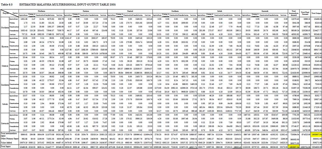
125 109

126 Table 6.1 Aggregated National Input-Output Table Malaysia 2005 (Million) Agriculture. Mining Construction Manufacturing Services Total Intermediate Demand Final Demand Total Output Agriculture 6, ,095 1,783 43,864 16,136 60,000 Mining ,601 37,720 1,567 41,508 53,902 95,410 Construction 8 1, ,163 16,452 24,417 36,653 61,070 Manufacturing 7,872 9,578 18, ,264 40, , , ,165 Services 3,668 5,765 8,712 75, , , , ,262 Sub-Total 18,372 17,446 29, , , , ,323 1,603,907 Other primary input 5,472 4,740 15, ,367 36, ,052 Value Added 36,156 73,224 15, , , ,271 Total Input 60,000 95,410 61, , ,262 1,603, ,323 1,603,

127 Table 6.3a to table 6.3f represented each region s intraregional block extracted from the MRIO table (table 6.0). The results were shown in the table 6.4 below. Then, the sum of each sector was compared to intermediate demand of the national input-output table. The differences are very small between and Table 6.3a Northern Region Sector Agriculture Mining Construction Manufacturing Services Agriculture Mining Construction Manufacturing Services Total Table 6.3b Eastern Region Sector Agriculture Mining Construction Manufacturing Services Agriculture Mining Construction Manufacturing Services Total Table 6.3c Central Region Sector Agriculture Mining Construction Manufacturing Services Agriculture Mining Construction Manufacturing Services Total

128 Table 6.3d Southern Region Sector Agriculture Mining Construction Manufacturing Services Agriculture Mining Construction Manufacturing Services Total Table 6.3e Sabah Region Sector Agriculture Mining Construction Manufacturing Services Agriculture Mining Construction Manufacturing Services Total Table 6.3f Sarawak Region Sector Agriculture Mining Construction Manufacturing Services Agriculture Mining Construction Manufacturing Services Total Comparison Intermediate Input Between MRIO Table and Table 6.4 National Input-Output Table Sector Agriculture Mining Construction Manufacturing Services Agriculture Mining Construction Manufacturing Services Total Intermediate Input National Input-Output Table Difference

129 1 1 3

130 6.2.2 Verification by Intermediate Demand Table 6.5 is partly extracted from the estimated MRIOT for the verification by intermediate demand. Table 6.6a to table 6.6f represented each region s intraregional transaction by intermediate demand extracted from the estimated MRIO table (table 6.0). For example, mining and quarrying sector, the figures from the Northern, the Eastern, Central, the Southern, Sabah, and Sarawak regions as shown in the rectangular boxes in table 6.5 were added up and the summary is shown in table 6.5a below: Table 6.5a Summary of Mining and Quarrying Sector Extracted from Table 6.5 for the Northern Region. Region Northern Sector Mining & quarrying Northern Eastern Central Southern Sabah Sarawak total The total 3.08 can be seen in a small rectangular box in table 6.6a. The rest of the sectors are derived in the same way. Table 6.6a Northern Region Sector Agriculture Mining Construction Manufacturing Services Total Agriculture Mining Construction Manufacturing Services Table 6.6b Eastern Region Sector Agriculture Mining Construction Manufacturing Services Total Agriculture Mining Construction Manufacturing Services

131 Table 6.6c Central Region Sector Agriculture Mining Construction Manufacturing Services Total Agriculture Mining Construction Manufacturing Services Table 6.6d Southern Region Sector Agriculture Mining Construction Manufacturing Services Total Agriculture Mining Construction Manufacturing Services Table 6.6e Sabah Region Sector Agriculture Mining Construction Manufacturing Services Total Agriculture Mining Construction Manufacturing Services Table 6.6f Sarawak Region Sector Agriculture Mining Construction Manufacturing Services Total Agriculture Mining Construction Manufacturing Services Like the verification by intermediate input, the sum of each sector is compared to intermediate demand of the national input-output table. The result is shown in table 6.7, and it is found that the differences are very small, between and

132 Table 6.7 Verification by Intermediate Demand: Comparison Between MRIO Table and National Input-Output Table Sector Agriculture Mining Construction Manufacturing Services Total Intermediate Demand National Input-output Table Difference Agriculture Mining Construction Manufacturing Services

133 6.2.3 Verification by Value Added The value added of each sector from each region in table 6.0 are added up and the total is compared with the national input-output table. The differences between the estimated MRIO and the national table are small, between and Table 6.8 Verification by Value Added Region Mining & Agriculture Construct Manufact Services Total Sector Quarrying Northern Eastern Central Southern Sabah Sarawak Total National Input-Output Table Difference Verification by Total Output Table 6.9 shows the extract total output of table 6.0. Each sector from each region is added up. For example, in the agricultural sector, the figures in the oval boxes from each region are added up to derive the total sum of 60,000 as shown in table 6.9a. Each sector from each region of the total output in table 6.0 are added up in the same way. Then, the total is compared with national input-output table. The results are shown in the table 6.9a and the differences are very small between and

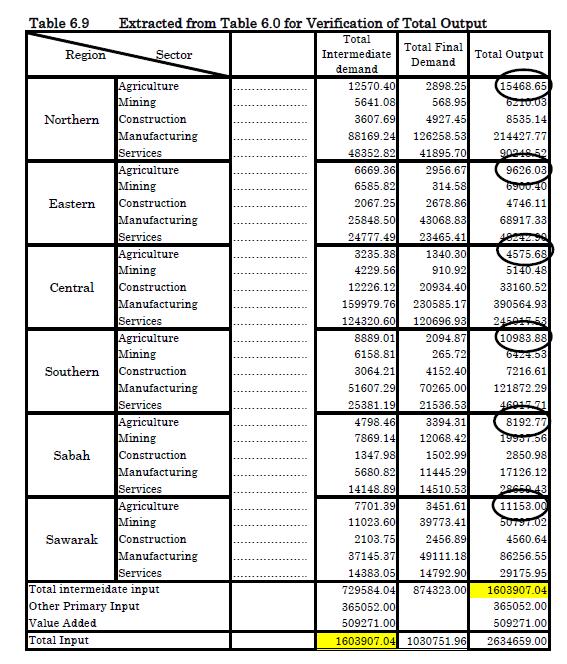
134 118

135 Table 6.9a Region Sector Verification by Total Output Northern Eastern Central Southern Sabah Sarawak Total National Input-Output Table Difference Agriculture Mining & Quarrying Construction Manufacturing Services

136 6.3 Analysis The estimated results show that different regions have different key sectors. This study identifies the key sector based on the following: i. Both values of the normalized indicators using backward and forward linkages are more than one; or ii. Both values of the weighted indicators using backward and forward linkages are more than one Share of Sectors in Region The table 6.10 below shows the share of all sectors in each region. These are the sum of the share of final demand of each region. It is indicated that the Central region has the highest share, 42.83% of the total final demand. The reasons is due to the fact that in this region the capital city of Malaysia, Kuala Lumpur, and other commercial centers are located. Another reason is this region is the most populated region with 8.2 million out of 26 millions total population in 2005 (see table 2.3). In contrast, Sabah region recorded 4.91%, lowest among the regions Share of Sector in Final Demand Table 6.10 shows that the final demand from the manufacturing sector is the highest in all the regions except in Sabah region where services sector contributes the highest, 1.66% share of the sector final demand. For East Malaysia (Sabah and Sarawak regions), mining and quarrying sector plays second in terms of share of the sector final demand, 1.38% and 4.55%, respectively. The other regions in the West Malaysia, mining and quarrying sector is the least important in the final demand Share of Sector in Value Added In table 6.10, the share of sector value added shows that services sector contributes the largest portion in the Northern with 7.97%, the Eastern with 4.78%, Central 22.45%, and the Southern regions with 4.16% compared to 120

137 Sabah with 3.19% and Sarawak regions, 3.11%. However, mining and quarrying sectors play an important role in the Sabah and Sarawak regions, with 3.26% and 10.57%, respectively. Table 6.10: Region Share of Sectors in the Region Share of Share of Sector in Sector sectors in Final region Demand Share of Sector in Value Added Agriculture 0.33% 1.18% Mining 0.07% 0.15% Northern Construction 0.56% 20.19% 0.42% Manufacturing 14.44% 5.97% Services 4.79% 7.97% Agriculture 0.34% 1.34% Mining 0.04% 0.09% Eastern Construction 0.31% 8.29% 0.25% Manufacturing 4.93% 3.12% Services 2.68% 4.78% Agriculture 0.15% 0.63% Mining 0.10% 0.24% Central Construction 2.39% 42.83% 1.71% Manufacturing 26.37% 13.61% Services 13.80% 22.45% Agriculture 0.24% 0.85% Mining 0.03% 0.07% Southern Construction 0.47% 11.24% 0.37% Manufacturing 8.04% 3.20% Services 2.46% 4.16% Agriculture 0.39% 1.57% Mining 1.38% 3.26% Sabah Construction 0.17% 4.91% 0.15% Manufacturing 1.31% 1.07% Services 1.66% 3.19% Agriculture 0.39% 1.53% Mining 4.55% 10.57% Sarawak Construction 0.28% 12.53% 0.21% Manufacturing 5.62% 2.78% Services 1.69% 3.11% 121

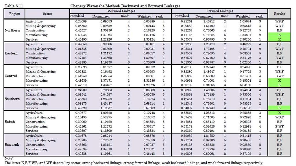
138 1 2 2

139 6.3.4 Chenery Watanabe Method (Direct Effect) This method measures only the first round effects generated from the relationship between the sectors based on direct input (or output) coefficients Analysis of Direct Backward Linkages In table 6.11, it is indicated that the normalized indicator shows that manufacturing sector has the highest direct backward linkage in all the regions except the Central region. These results show the same for the Rasmussen method (see table 6.12). Construction sector has the highest direct effect in the Central region but second in the Northern, Eastern, Southern and Sarawak regions. During the eighth Malaysia Plan, the Malaysian government has encouraged the private sectors to develop infrastructures and spread more industries throughout the country. The state of Pulau Pinang (Northern region) and the states of Selangor, Negeri Sembilan, and Melaka (Central region) are industrial zone. The expansion of contractor sector was attributed to the civil engineering activities which were related to the development of manufacturing sector. Thus, manufacturing and construction sectors have strong backward linkage in these regions. Moreover, the Central region is the commercial centers. The agricultural sector has less direct effect in all regions except Sabah which ranked second and become the key sector of this region. During the seventh Malaysia Plan, under the land utilization scheme, agricultural land usage has increased from 5.7 million hectares in 1995 to 6 million hectares in 2000, mainly due to the opening of new land for oil palm cultivation in the Sabah region, besides the increased in hectares for vegetables, fruits and tobacco (Malaysia, 2001). These are amongst the factors that contributed to the strong direct effect of agricultural sector in the Sabah region. Meanwhile, the service sector shows similar results in all the regions and it ranked fourth amongst the sectors. The least direct effect is mining and quarrying sector and this can be seen in all regions. Weighted indicator also indicated that manufacturing sector is the highest rank in the pull effect in all regions. The agricultural sector is in the fourth 123

140 rank in all the regions. Meanwhile, construction sector shows the lowest rank in Sabah and Sarawak regions. The main reason is that these regions are large and the population density is very small to carry out and develop the construction sector. Sarawak is the largest state which covers 124,450 square kilometers with the population density of only 18 people. Sabah is the second largest in Malaysia after Sarawak which covers 73,620 square kilometers with the population density of 42 people (see table 2.3). The other reason is due to its hard infrastructure (road, ports, electricity, water and data connectivity) and soft infrastructure (human capital) which are lagged behind from the rest of Malaysia The mining and quarrying sector is also less important in the Northern, Eastern, Central, and Southern regions because in these regions, economic activities are concentrated more in the manufacturing and services sectors. Nevertheless, it shows a higher pull effect in the regions of Sabah and Sarawak, third and second ranked, respectively because in these regions there are plenty of natural resources. For example, the exploration of Petroleum in Sarawak has begun in the early 20 th century where oil was first discovered in 1909 and first produced in 1910 (Razmahwata, 2005). In the state of Sabah there are many river sand and stone mining activities and currently the total length of river which is affected by the project is estimated at 808 kilometers throughout the state (SECD, 2000). Thus, these regions have a strong direct effect in mining and quarrying sector Analysis of Forward Linkages In table 6.11, with Normalized indicators show that mining and quarrying sector has the highest direct forward linkage in the Northern, Eastern, Central, and Southern regions. This sector has the least push effect in Sarawak and Sabah regions. Construction sector is unimportant in the Northern, Eastern, and Central regions. Nevertheless, it is fairly important which ranked third in Sabah and Sarawak regions where is ranked third. Weighted indicator shows that the service sector has the highest direct effect in all the regions except Sarawak region. Construction sector shows the 124

141 least important in all regions. Agricultural sector shows fairly important in the Northern, Southern, and Sabah regions. This sector does not play an important role in the Central and Sarawak regions. Most of the states in the Central region concentrated more on manufacturing and services sectors. Sarawak s agricultural activity is characterized by low productivity and decreasing output relative to other sectors. Although a large sum of money was allocated to develop the agricultural sector in Sarawak over many Malaysia Plans, the development is not as expected. The agricultural programs are not fully understood by the smallholders and also due to the poor condition of hard and soft infrastructure as mentioned above and these could not support the agricultural sector to growth. Mining and quarrying sector has the highest rank in Sarawak region and it is in the second rank in Sabah and in the other regions hence, it is fairly important Rasmussen Method (Direct and Indirect Effect) This method measures the intersectoral linkages by taking into account both direct and indirect effects generated by the interrelationships between the sectors in the economy. The backward linkage is measured by the columns sum of the Leontief s inverse matrix, whereas the forward linkage is measured by the row sum of Ghosh s inverse matrix Analysis of Backward Linkages (Power of Dispersion Index) Table 6.12 shows that with normalized indicator, manufacturing sector plays the most important role in economy for all the regions except the Central region. In the Central region, construction sector has the most important pull effect. The construction sector is ranked second pull effect to other regions such as in the Northern, Eastern, Southern, and Sarawak. The agricultural sector is unimportant in all the regions except for Sabah region, where this sector ranked second, as less pull effect to other sectors in the economy. The least important of pull effect in all the regions is mining and quarrying sector. 125

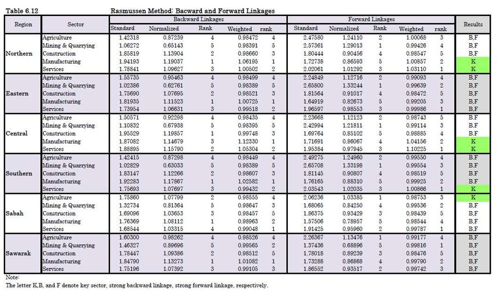
142 1 2 6

143 The weighted indicator confirmed that the manufacturing sector has the most pull effect. Agricultural sector ranked second least pull effect in all the regions. Mining and quarrying sector has the least pull effect in the Northern, Eastern, Central, and Southern regions and fairly important in Sabah region but ranked second in Sarawak region. Construction sector is fairly important in the Northern, Eastern and Central regions and the least pull effect in the Sabah and Sarawak regions Analysis of Forward Linkages (Sensitivity Dispersion Index) The normalized indicator shows that the agricultural sector has the most push effect in the Sabah and Sarawak regions and its role is also important in the rest of the regions. The manufacturing sector has the least push effect in the Northern, Eastern, Southern regions and is ranked second in the Central and Sarawak regions. Two regions, Sabah and Sarawak show that the services sector plays second after agriculture as the most push effect. The Northern, Eastern, and Southern regions show third rank in the list of push effect. Mining and quarrying sector has the highest push effect in the Northern, Eastern, Southern, and Sabah regions and the fourth rank in the Central and Sarawak regions. Services sector is fairly important as push effect in the Northern, Eastern, and Central regions but its role is important in Sabah and Sarawak regions. From the results of the weighted indicators, services sector has the most push effect in all regions except in the Sarawak region. Construction sector has the least push effect in all the regions. Table 6.12 shows manufacturing sector has ranked second as the push effect in four regions; Northern, Central, Southern and Sarawak regions. It is not important in Sabah region but fairly important as push effect in the Eastern region. Mining and quarrying sector is important as push effect in the Eastern, Sabah and Sarawak regions, fairly important in Eastern and Central regions and least important in the Northern region. Agricultural sector has the least push effect in four 127

144 regions; Eastern, Central, Southern, and Sarawak regions and fairly important in the Northern and Sabah regions. 6.4 Conclusion Based on the verification of the estimated MRIO table, it could be concluded that it is acceptable and a reliable method to be used to identify the key sector of the regions with small discrepancy from the national input-output table. Generally, the linkage analysis results show that the manufacturing sector has the strong backward and forward linkages in all the regions. These results are consistent with the analysis done on the national input-output table in chapter four which revealed the manufacturing and services sector are the key sectors. In terms of ranking, both Chenery-Watanabe and Rasmussen methods, backward and forward linkages, normalized and weighted indicators indicated the same rank but with different values. This indicated that the two methods are also consistent to each other. Based on Chenery-Watanabe method (Table 6.11) and Rasmussen method (Table 6.12), the key sectors for the Northern and Central regions are manufacturing and services sectors. Agricultural sector is the key sector for Sabah region. The key sector for the Southern region is the services sector with normalized indicator using Rasmussen method and has stronger backward and forward linkages with weighted indicator as well as using the Chenery-Watanabe method. There is no key sector in the Eastern and Sarawak regions but both have strong backward and forward linkages. Table 6.13 shows the summary of interregional key sectors which have been identified for 2005 based on the estimated MRIO table (see table 6.0). Table 6.13 also depicted the government efforts to enhance the regional economy by the introduction of special economic corridor for each region with exception to the Central region. The Central region is the most developed 128

145 amongst the regions where it is the economy hub of the nation, cosmopolitan cities and where the main governmental offices are located. The infrastructures are well constructed and many industrial zones are created. The key sectors for the Northern and Central are consistent with the national key sectors in this study. The Central region contributed 41% of the national GDP in 2005 with manufacturing and services sectors as major contributors. Among the states in the Central region, the Selangor state contributed the largest share, 23% of the national GDP in 2005 because this state is in the industrial zone. Out of the 23% share, the manufacturing and services sectors contributed 53.5% and 41.2% respectively (Malaysia, 2006). The manufacturing sectors in the Northern region are concentrated more in the Pulau Pinang state. In 2005, the manufacturing sector in Pulau Pinang state contributed 54% to the state s GDP with diversified industries such as Electrical and Electronics, medical supplies, and food processing. The contribution of service sectors of this state is also significant to Pulau Pinang s GDP which was 41% in According to Department of Statistics, the two biggest contributors to the service sectors are finance, insurance, real estate and business services sectors and wholesale, retail trade, accommodation and restaurant. Meanwhile, the agricultural sector in the Eastern region contributed 11.5% to the national GDP (Malaysia, 2006). The role of agricultural sector in this region is significant to the national GDP although it is not a key sector. The Eastern region has strong backward and forward linkage in agricultural, construction and services sectors. Basically, the Eastern region is rich in agricultural resources, rubber, and fisheries. In early 1980 s, this sector was the main contributor to region s GDP. However, in 1990 s the diversification of economic activities were implemented and agricultural sector became third largest contributor to the region s GDP after manufacturing and services sectors. Nevertheless, the performance of the manufacturing and services sectors are still far behind the Northern region (Hassan et al., 2011). Table 6.13, ECERDC has identified the potential projects to strengthen the region s, 129

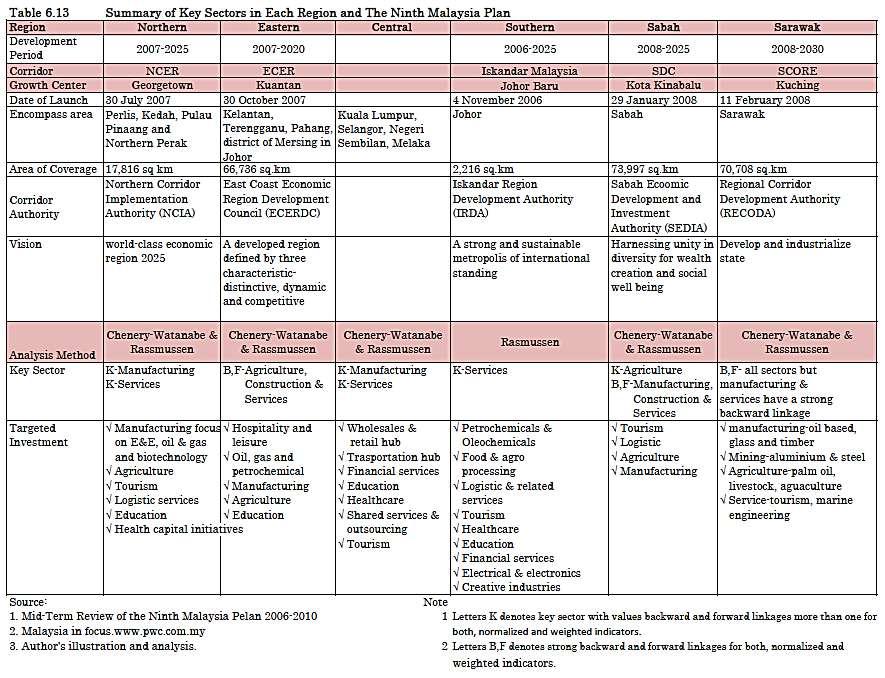
146 1 3 0